TABLE 6.26 Sensors and Manufacturers

7.Nonvolatile Electronics Inc. NVSB series datasheet. March 1996.

8.J. R. Carstens, Electrical Sensors and Transducers, Englewood Cliffs, NJ: Regents/Prentice-Hall, 1992, p. 125.

9.H. Norton, Handbook of Transducers, Englewood Cliffs, NJ: Prentice-Hall, 1989, 106-112.

Further Information

B. D. Cullity, Introduction to Magnetic Materials, Reading, MA: Addison-Wesley, 1972. D. Craik, Magnetism Principles and Applications, New York: John Wiley & Sons, 1995.

P. Lorrain and D. Corson, Electromagnetic Fields and Waves, San Francisco: W.H. Freeman, 1962. R. Boll, Soft Magnetic Materials, London: Heyden & Son, 1977.

H. Olson, Dynamical Analogies, New York: D. Van Nostrand, 1943.

D. Askeland, The Science and Engineering of Materials, Boston: PWS-Kent Publishing, 1989.

R. Rose, L. Shepard, and J. Wulff, The Structure and Properties of Materials, New York: John Wiley & Sons, 1966.

J. Shackelford, Introduction to Materials Science for Engineers, New York: Macmillan, 1985.

D.Jiles, Introduction to Magnetism and Magnetic Materials, London: Chapman and Hall, 1991.

F.Mazda, Electronics Engineer’s Reference Book, 6th ed., London: Butterworth, 1989.

E.Herceg, Handbook of Measurement and Control, New Jersey: Schaevitz Engineering, 1976.

6.10 Synchro/Resolver Displacement Sensors

Robert M. Hyatt, Jr. and David Dayton

Most electromagnetic position transducers are based on transformer technology. Transformers work by exciting the primary winding with a continuously changing voltage and inducing a voltage in the secondary winding by subjecting it to the changing magnetic field set up by the primary. They are aconly devices, which make all electromagnetically coupled position sensors ac transformer coupled. They are inductive by nature, consisting of wound coils. By varying the amount of coupling from the primary (excited) winding of a transformer to the secondary (coupled) winding with respect to either linear or rotary displacement, an analog signal can be generated that represents the displacement. This coupling variation is accomplished by moving either one of the windings or a core element that provides a flux path between the two windings.

© 1999 by CRC Press LLC

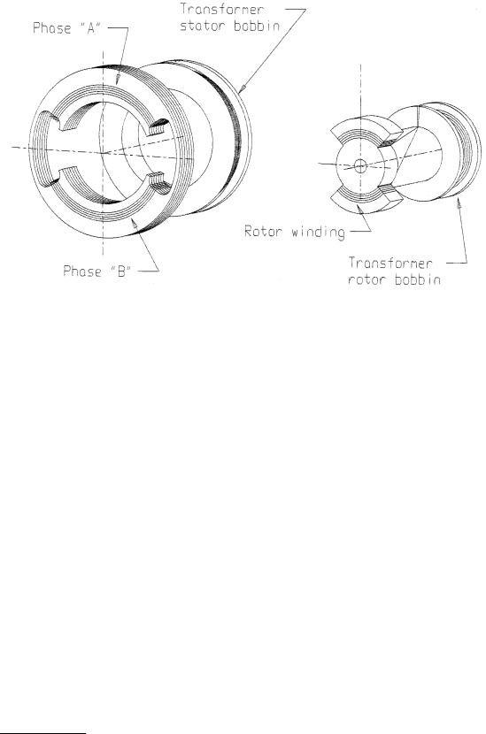
FIGURE 6.89 The induction potentiometer has windings on the rotor and the stator.

One of the simplest forms of electromagnetic position transducers is the LVDT, which is described in Section 6.2 on inductive sensors. If the displacement of the core in an LVDT-type unit is changed from linear to rotary, the device becomes an RVDT (rotary variable differential transformer).

Induction Potentiometers

The component designer can “boost” the output, increase accuracy, and achieve a slightly greater angular range if windings are placed on the rotor as shown in Figure 6.89. The disadvantages to this method are

(1) additional windings, (2) more physical space required, (3) greater variation over temperature, and

(4) greater phase shift due to the additional windings.

The advantage of the induction pot design is greater sensitivity (more volts per degree), resulting in better signal to noise and higher accuracy in most cases.

Resolvers

If the two-slot lamination in the stator stack shown in Figure 6.89 is replaced by a multislot lamination (see Figure 6.90), and two sets of windings are designed in concentric coil sets and distributed in each quadrant of the laminated stack; a close approximation to a sine wave can be generated on one of the secondary windings and a close approximation to a cosine wave can be generated on the other set of windings. Rotary transformers of this design are called resolvers. Using a multislot rotor lamination and distributing the windings in the rotor, the sine-cosine waveforms can be improved even further.

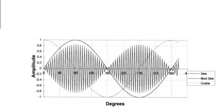
A resolver effectively amplitude modulates the ac excitation signal placed on the rotor windings in proportion to the sine and the cosine of the angle of mechanical rotation. This sine-cosine electrical output information measured across the stator windings may be used for position and velocity data. In this manner, the resolver is an analog trigonometric function generator. Most resolvers have two primary windings that are located at right angles to each other in the stator, and two secondary windings also at right angles to each other, located on the rotor (see Figure 6.91).

© 1999 by CRC Press LLC

FIGURE 6.90 The resolver stator has distributed coil windings on a 16-slot lamination to generate a sine wave.

FIGURE 6.91 A brushless resolver modulates the ac excitation on the rotor by the rotation angle.

If the rotor winding (R1-R3) is excited with the rated input voltage (see Figure 6.92), the amplitude of the output winding of the stator (S2-S4) will be proportional to the sine of the rotor angle θ, and the amplitude of the output of the second stator winding (S1-S3) will be proportional to cosine θ. (See Figure 6.93.) This is commonly called the “control transmitter” mode and is used with most “state-of- the-art” resolver to digital converters.

In the control transmitter mode, electrical zero may be defined as the position of the rotor with respect to the stator at which there is minimum voltage across S2-S4 when the rotor winding R1-R3 is excited

© 1999 by CRC Press LLC

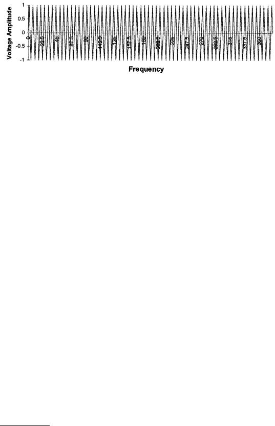
FIGURE 6.92 The resolver rotor winding is excited with the rated input voltage.

with rated voltage. Nulls will occur across S2-S4 at the 0° and 180° positions, and will occur across S1-S3 at the 90° and 270° positions.

If the stator winding S1-S3 is excited with the rated input voltage and stator winding S2-S4 is excited with the rated input voltage electrically shifted by exactly 90°, then the output sensed on the rotor winding R1-R3 does not vary with rotor rotation in amplitude or frequency from the input reference signal. It is the sum of both inputs. It does, however, vary in time phase from the rated input by the angle of the shaft from a referenced “zero” point (see Figure 6.94). This is a “phase analog” output and the device is termed a “control transformer.” By measuring the time difference between the zero crossing of the reference voltage waveform and the output voltage waveform, the phase angle (which is the physical angular displacement of the output shaft) can be calculated.

Because the resolver is an analog device and the outputs are continuous through 360°, the theoretical resolution of a resolver is infinite. There are, however, ambiguities in output voltages caused by inherent variations in the transformation of the voltage from primary to secondary through 360° of rotation. These ambiguities result in inaccuracy when determining the true angular position. The types of error signals that are found in resolvers are shown in Figure 6.95.

As a rule, the larger the diameter of the stator laminations, the better the accuracy and the higher the absolute resolution of the device. This is a function of the number of magnetic poles that can be fit into the device, which is a direct function of the number of slots in the stator and rotor laminations. With multispeed units (see the section on multispeeds below), the resolution increases as a multiple of the speeds. For most angular excursions, the multispeed resolver can exceed the positioning accuracy capability of any other component in its size, weight, and price range.

Operating Parameters and Specifications for Resolvers

There are seven functional parameters that define the operation of a resolver in the analog mode. These are (1) accuracy, (2) operating voltage amplitude, (3) operating frequency, (4) phase shift of the output voltage from the referenced input voltage, (5) maximum allowable current draw, (6) the transformation ratio of output voltage over input voltage, and (7) the null voltage. Although impedance controls the functional parameters, it is transparent to the user. The lamination and coil design are usually developed to minimize null voltage and input current, and the impedance is a direct fallout of the inherent design of the resolver. The following procedure can be used to measure the seven values for most resolvers.

Equipment Needed for Testing Resolvers

A mechanical index stand that can position the shaft of the resolver to an angular accuracy that is an order of magnitude greater than the specified accuracy of the resolver.

An ac signal generator capable of up to 24 Vrms at 10 kHz.

A phase angle voltmeter (PAV) capable of measuring “in phase” and “quadrature” voltage components for determining the transformation ratio and the null voltage as well as the phase angle between the output voltage and the reference input voltage.

A 1 Ω resistor used to measure input current with the PAV.

© 1999 by CRC Press LLC

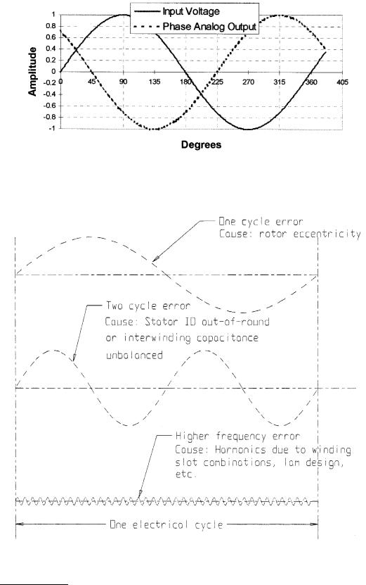
FIGURE 6.94 Resolver stator windings excited at 0° and 90° yield a phase shift with rotor rotation. Phase analog output at 225° vs. input voltage.

FIGURE 6.95 There are several causes of errors in resolvers and synchros.

© 1999 by CRC Press LLC

An angle position indicator (API) used in conjunction with the index stand to measure the accuracy of the resolver.

1.Using the above equipment with the index stand in the 0° position, mount the resolver on the index stand and lock the resolver shaft in place.

2.Place the 1 Ω resistor in series with the R1 (red/wht) lead of the resolver.

3.Connect the resolver rotor leads, R1 (red/wht) & R3 (yel/wht) (see Figure 6.91) to the sine wave signal generator and set the voltage and frequency to the designed values for the resolver.

4.Connect the terminals from the sine wave signal generator to the reference input of the phase angle voltmeter (PAV).

5.Connect the resolver output leads S2 (yel) and S4 (blu) to the PAV input terminals and place the PAV in the total output voltage mode.

6.Rotate the index stand to the 0° position.

7.Turn the resolver housing while monitoring the total output voltage on the PAV until a minimum voltage reading is obtained on the PAV. Record this value. This is the null voltage of the resolver.

8.Turn the index stand to the 90° position.

9.Change the output display on the PAV to show the phase angle between the reference voltage and the voltage on leads S2-S4. Record this phase angle reading.

10.Change the output display on the PAV to show the total output voltage of the resolver.

11.Record this voltage.

12.Calculate the transformation ratio by dividing the reading in step 11 by the input reference voltage amplitude.

13.Connect the input leads of the PAV across the 1 Ω resistor and record the total voltage on the PAV display. Since this reading is across a 1 Ω resistor, it is also the total current.

14.Disconnect the resolver and the signal generator from the PAV.

15.Connect the terminals from the sine wave signal generator to the reference input of the angle position indicator (API).

16.Connect the stator leads S1 (red), S3 (blk), S2 (yel), and S4 (blu) to the API S1, S3, S2, and S4 inputs, respectively.

17.Check the accuracy of the resolver by recording the display on the API every 20° through 360° of mechanical rotation on the index stand. Record all values.

Resolver Benefits

Designers of motion control systems today have a variety of technologies from which to choose feedback devices. The popularity of brushless dc motors has emphasized the need for rotor position information to commutate windings as a key application in sensor products. Encoders are widely used due to the ease of interface with today’s drivers but have some inherent performance limitations in temperature range, shock and vibration handling, and contamination resistance. The resolver is a much more rugged device due to its construction and materials, and can be mated with modular R to D converters that will meet all performance requirements and work reliably in the roughest of industrial and aerospace environments.

The excitation signal Ex into the resolver is converted by transformer coupling into sine and cosine (quadrature) outputs which equal Exsin θ and Excos θ. The resolver-to-digital converter (shown in Figure 6.98) calculates the angle:

In this ratiometric format, the output of the sine winding is divided by the output of the cosine winding, and any injected noise whose magnitude is approximately equivalent on both windings is canceled. This provides an inherent noise rejection feature that is beneficial to the resolver user. This feature also results in a large degree of temperature compensation.

© 1999 by CRC Press LLC