Frequency

Measurement

19.1Overview of Frequency Measurements and Calibration

19.2The Specifications: Frequency Uncertainty and

Stability

Frequency Uncertainty • Stability

19.3Frequency Standards

Quartz Oscillators • Atomic Oscillators

Frequency is the rate of occurrence of a repetitive event. If T is the period of a repetitive event, then the frequency f = 1/T. The International System of Units (SI) states that the period should always be expressed in units of seconds (s), and the frequency should always be expressed in hertz (Hz). The frequency of electric signals often is measured in units of kilohertz (kHz) or megahertz (MHz), where 1 kHz equals 1000 (103) cycles per second, and 1 MHz equals 1 million (106) cycles per second.

Average frequency over a time interval can be measured very precisely. Time interval is one of the four basic standards of measurement (the others are length, mass, and temperature). Of these four basic standards, time interval (and frequency) can be measured with the most resolution and the least uncertainty. In some fields of metrology, 1 part per million (1 × 10–6) is considered quite an accomplishment. In frequency metrology, measurements of 1 part per billion (1 × 10–9) are routine, and even 1 part per trillion (1 × 10–12) is commonplace.

Devices that produce a known frequency are called frequency standards. These devices must be calibrated so that they remain within the tolerance required by the user’s application. The discussion begins with an overview of frequency calibrations.

19.1 Overview of Frequency Measurements and Calibration

Frequency calibrations measure the performance of frequency standards. The frequency standard being calibrated is called the device under test (DUT). In most cases, the DUT is a quartz, rubidium, or cesium oscillator. In order to perform the calibration, the DUT must be compared to a standard or reference. The standard should outperform the DUT by a specified ratio in order for the calibration to be valid. This ratio is called the test uncertainty ratio (TUR). A TUR of 10:1 is preferred, but not always possible. If a smaller TUR is used (5:1, for example), then the calibration will take longer to perform.

© 1999 by CRC Press LLC

Once the calibration is completed, the metrologist should be able to state how close the DUT’s output is to its nameplate frequency. The nameplate frequency is labeled on the oscillator output. For example, a DUT with an output labeled “5 MHz” is supposed to produce a 5 MHz frequency. The calibration measures the difference between the actual frequency and the nameplate frequency. This difference is called the frequency offset. There is a high probability that the frequency offset will stay within a certain range of values, called the frequency uncertainty. The user specifies a frequency offset and an associated uncertainty requirement that the DUT must meet or exceed. In many cases, users base their requirements on the specifications published by the manufacturer. In other cases, they may “relax” the requirements and use a less demanding specification. Once the DUT meets specifications, it has been successfully calibrated. If the DUT cannot meet specifications, it fails calibration and is repaired or removed from service.

The reference used for the calibration must be traceable. The International Organization for Standardization (ISO) definition for traceability is:

The property of the result of a measurement or the value of a standard whereby it can be related to stated references, usually national or international standards, through an unbroken chain of comparisons all having stated uncertainties [1].

In the United States, the “unbroken chain of comparisons” should trace back to the National Institute of Standards and Technology (NIST). In some fields of calibration, traceability is established by sending the standard to NIST (or to a NIST-traceable laboratory) for calibration, or by sending a set of reference materials (such as a set of artifact standards used for mass calibrations) to the user. Neither method is practical when making frequency calibrations. Oscillators are sensitive to changing environmental conditions and especially to being turned on and off. If an oscillator is calibrated and then turned off, the calibration could be invalid when the oscillator is turned back on. In addition, the vibrations and temperature changes encountered during shipment can also change the results. For these reasons, laboratories should make their calibrations on-site.

Fortunately, one can use transfer standards to deliver a frequency reference from the national standard to the calibration laboratory. Transfer standards are devices that receive and process radio signals that provide frequency traceable to NIST. The radio signal is a link back to the national standard. Several different types of signals are available, including NIST radio stations WWV and WWVB, and radionavigation signals from LORAN-C and GPS. Each signal delivers NIST traceability at a known level of uncertainty. The ability to use transfer standards is a tremendous advantage. It allows traceable calibrations to be made simultaneously at a number of sites as long as each site is equipped with a radio receiver. It also eliminates the difficult and undesirable practice of moving frequency standards from one place to another.

Once a traceable transfer standard is in place, the next step is developing the technical procedure used to make the calibration. This procedure is called the calibration method. The method should be defined and documented by the laboratory, and ideally a measurement system that automates the procedure should be built. ISO/IEC Guide 25, General Requirements for the Competence of Calibration and Testing Laboratories, states:

The laboratory shall use appropriate methods and procedures for all calibrations and tests and related activities within its responsibility (including sampling, handling, transport and storage, preparation of items, estimation of uncertainty of measurement, and analysis of calibration and/or test data). They shall be consistent with the accuracy required, and with any standard specifications relevant to the calibrations or test concerned.

In addition, Guide 25 states:

The laboratory shall, wherever possible, select methods that have been published in international or national standards, those published by reputable technical organizations or in relevant scientific texts or journals [2,3].

© 1999 by CRC Press LLC

Calibration laboratories, therefore, should automate the frequency calibration process using a welldocumented and established method. This helps guarantee that each calibration will be of consistently high quality, and is essential if the laboratory is seeking ISO registration or laboratory accreditation.

Having provided an overview of frequency calibrations, we can take a more detailed look at the topics introduced. This chapter begins by looking at the specifications used to describe a frequency calibration, followed by a discussion of the various types of frequency standards and transfer standards. A discussion of some established calibration methods concludes this chapter.

19.2The Specifications: Frequency Uncertainty and Stability

This section looks at the two main specifications of a frequency calibration: uncertainty and stability.

Frequency Uncertainty

As noted earlier, a frequency calibration measures whether a DUT meets or exceeds its uncertainty requirement. According to ISO, uncertainty is defined as:

Parameter, associated with the result of a measurement, that characterizes the dispersion of values that could reasonably be attributed to the measurand [1].

When we make a frequency calibration, the measurand is a DUT that is supposed to produce a specific frequency. For example, a DUT with an output labeled 5 MHz is supposed to produce a 5 MHz frequency. Of course, the DUT will actually produce a frequency that is not exactly 5 MHz. After calibration of the DUT, we can state its frequency offset and the associated uncertainty.

Measuring the frequency offset requires comparing the DUT to a reference. This is normally done by making a phase comparison between the frequency produced by the DUT and the frequency produced by the reference. There are several calibration methods (described later) that allow this determination. Once the amount of phase deviation and the measurement period are known, we can estimate the frequency offset of the DUT. The measurement period is the length of time over which phase comparisons are made. Frequency offset is estimated as follows, where t is the amount of phase deviation and T is the measurement period:

If we measure +1 µs of phase deviation over a measurement period of 24 h, the equation becomes:

The smaller the frequency offset, the closer the DUT is to producing the same frequency as the reference. An oscillator that accumulates +1 µs of phase deviation per day has a frequency offset of about –1 × 10–11 with respect to the reference. Table 19.1 lists the approximate offset values for some standard units of phase deviation and some standard measurement periods.

The frequency offset values in Table 19. 1 can be converted to units of frequency (Hz) if the nameplate frequency is known. To illustrate this, consider an oscillator with a nameplate frequency of 5 MHz that is high in frequency by 1.16 × 10–11. To find the frequency offset in hertz, multiply the nameplate frequency by the dimensionless offset value:

© 1999 by CRC Press LLC

TABLE 19. 1 Frequency Offset Values for Given

Amounts of Phase Deviation

The nameplate frequency is 5 MHz, or 5,000,000 Hz. Therefore, the actual frequency being produced by the frequency standard is:

To do a complete uncertainty analysis, the measurement period must be long enough to ensure that one is measuring the frequency offset of the DUT, and that other sources are not contributing a significant amount of uncertainty to the measurement. In other words, must be sure that t is really a measure of the DUT’s phase deviation from the reference and is not being contaminated by noise from the reference or the measurement system. This is why a 10:1 TUR is desirable. If a 10:1 TUR is maintained, many frequency calibration systems are capable of measuring a 1 × 10–10 frequency offset in 1 s [4].

Of course, a 10:1 TUR is not always possible, and the simple equation given for frequency offset (Equation 19.1) is often too simple. When using transfer standards such as LORAN-C or GPS receivers (discussed later), radio path noise contributes to the phase deviation. For this reason, a measurement period of at least 24 h is normally used when calibrating frequency standards using a transfer standard. This period is selected because changes in path delay between the source and receiver often have a cyclical variation that averages out over 24 h. In addition to averaging, curve-fitting algorithms and other statistical methods are often used to improve the uncertainty estimate and to show the confidence level of the measurement [5]. Figure 19.1 shows two simple graphs of phase comparisons between a DUT and a reference frequency. Frequency offset is a linear function, and the top graph shows no discernible variation in the linearity of the phase. This indicates that a TUR of 10:1 or better is being maintained. The bottom graph shows a small amount of variation in the linearity, which could mean that a TUR of less than 10:1 exists and that some uncertainty is being contributed by the reference.

To summarize, frequency offset indicates how accurately the DUT produces its nameplate frequency. Notice that the term accuracy (or frequency accuracy) often appears on oscillator specification sheets instead of the term frequency offset, since frequency accuracy and frequency offset are nearly equivalent terms. Frequency uncertainty indicates the limits (upper and lower) of the measured frequency offset. Typically, a 2σ uncertainty test is used. This indicates that there is a 95.4% probability that the frequency offset will remain within the stated limits during the measurement period. Think of frequency offset as the result of a measurement made at a given point in time, and frequency uncertainty as the possible dispersion of values over a given measurement period.

Stability

Before beginning a discussion of stability, it is important to mention a distinction between frequency offset and stability. Frequency offset is a measure of how well an oscillator produces its nameplate frequency, or how well an oscillator is adjusted. It does not tell us about the inherent quality of an oscillator. For example, a high-quality oscillator that needs adjustment could produce a frequency with

© 1999 by CRC Press LLC

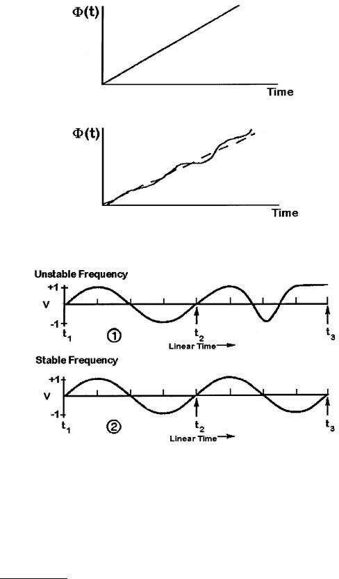
FIGURE 19.1 Simple phase comparison graphs.

FIGURE 19.2 Comparison of unstable and stable frequencies.

a large offset. A low-quality oscillator may be well adjusted and produce (temporarily at least) a frequency very close to its nameplate value.

Stability, on the other hand, indicates how well an oscillator can produce the same frequency over a given period of time. It does not indicate whether the frequency is “right” or “wrong,” only whether it stays the same. An oscillator with a large frequency offset could still be very stable. Even if one adjusts the oscillator and moves it closer to the correct frequency, the stability usually does not change. Figure 19.2 illustrates this by displaying two oscillating signals that are of the same frequency between t1 and t2. However, it is clear that signal 1 is unstable and is fluctuating in frequency between t2 and t3.

© 1999 by CRC Press LLC

Stability is defined as the statistical estimate of the frequency fluctuations of a signal over a given time interval. Short-term stability usually refers to fluctuations over intervals less than 100 s. Long-term stability can refer to measurement intervals greater than 100 s, but usually refers to periods longer than 1 day. A typical oscillator specification sheet might list stability estimates for intervals of 1, 10, 100, and 1000 s [6, 7].

Stability estimates can be made in the frequency domain or time domain, but time domain estimates are more widely used. To estimate stability in the time domain, one must start with a set of frequency offset measurements yi that consists of individual measurements, y1, y2, y3, etc. Once this dataset is obtained, one needs to determine the dispersion or scatter of the yi as a measure of oscillator noise. The larger the dispersion, or scatter, of the yi, the greater the instability of the output signal of the oscillator.

Normally, classical statistics such as standard deviation (or variance, the square of the standard deviation) are used to measure dispersion. Variance is a measure of the numerical spread of a dataset with respect to the average or mean value of the data set. However, variance works only with stationary data, where the results must be time independent. This assumes the noise is white, meaning that its power is evenly distributed across the frequency band of the measurement. Oscillator data is usually nonstationary, because it contains time-dependent noise contributed by the frequency offset. For stationary data, the mean and variance will converge to particular values as the number of measurements increases. With nonstationary data, the mean and variance never converge to any particular values. Instead, there is a moving mean that changes each time a new measurement is added.

For these reasons, a nonclassical statistic is used to estimate stability in the time domain. This statistic is often called the Allan variance; but because it is actually the square root of the variance, its proper name is the Allan deviation. By recommendation of the Institute of Electrical and Electronics Engineers (IEEE), the Allan deviation is used by manufacturers of frequency standards as a standard specification for stability. The equation for the Allan deviation is:

where M is the number of values in the yi series, and the data are equally spaced in segments τ seconds long. Note that while classical deviation subtracts the mean from each measurement before squaring their summation, the Allan deviation subtracts the previous data point. Since stability is a measure of frequency fluctuations and not of frequency offset, the differencing of successive data points is done to

–

remove the time-dependent noise contributed by the frequency offset. Also, note that the y values in the equation do not refer to the average or mean of the dataset, but instead imply that the individual measurements in the dataset are obtained by averaging.

Table 19.2 shows how stability is estimated. The first column is a series of phase measurements recorded at 1 s intervals. Each measurement is larger than the previous measurement. This indicates that the DUT is offset in frequency from the reference and this offset causes a phase deviation. By differencing the raw phase measurements, the phase deviations shown in the second column are obtained. The third column divides the phase deviation ( t) by the 1 s measurement period to get the frequency offset. Since the phase deviation is about 4 ns s–1, it indicates that the DUT has a frequency offset of about 4 × 10–9. The frequency offset values in the third column form the yi data series. The last two columns show the first differences of the yi and the squares of the first differences. Since the sum of the squares equals 2.2 × 10–21, the equation (where τ = 1 s) becomes:

© 1999 by CRC Press LLC