


less common, and more expensive. Receivers range in price from less than $100 for an OEM timing board, to $20,000 or more for the most sophisticated models. The price often depends on the quality of the receiver’s timebase oscillator. Lower priced models have a low-quality timebase that must be constantly steered to follow the GPS signal. Higher priced receivers have better timebases (some have internal rubidium oscillators) and can ignore many of the GPS path variations because their oscillator allows them to coast for longer intervals [21].
Most GPS receivers provide a 1 pulse per second (pps) output. Some receivers also provide a 1 kHz output (derived from the C/A code) and at least one standard frequency output (1, 5, or 10 MHz). To use these receivers, one simply mounts the antenna, connects the antenna to the receiver, and turns the receiver on. The antenna is often a small cone or disk (normally about 15 cm in diameter) that must be mounted outdoors where it has a clear, unobstructed view of the sky. Once the receiver is turned on, it performs a sky search to find out which satellites are currently above the horizon and visible from the antenna site. It then computes its three-dimensional coordinate (latitude, longitude, and altitude as long as four satellites are in view) and begins producing a frequency signal. The simplest GPS receivers have just one channel and look at multiple satellites using a sequencing scheme that rapidly switches between satellites. More sophisticated models have parallel tracking capability and can assign a separate channel to each satellite in view. These receivers typically track from 5 to 12 satellites at once (although more than 8 will only be available in rare instances). By averaging data from multiple satellites, a receiver can remove some of the effects of SA and reduce the frequency uncertainty.
GPS Performance
GPS has many technical advantages over LORAN-C. The signals are usually easier to receive, the equipment is often less expensive, and the coverage area is much larger. In addition, the performance of GPS is superior to that of LORAN-C. However, like all transfer standards, the short-term stability of a GPS receiver is poor (made worse by SA), and it lengthens the time required to make a calibration. As with LORAN-C, a measurement period of at least 24 h is recommended when calibrating atomic frequency standards using GPS.
To illustrate this, Figure 19.8 shows a 100 s comparison between GPS and a cesium oscillator. The cesium oscillator has a frequency offset of 1 × 10–13, and its accumulated phase shift during the 100 s measurement period is <1 ns. Therefore, the noise on the graph can be attributed to GPS path variations and SA.
Figure 19.9 shows a 1-week comparison between a GPS receiver and the same cesium oscillator used in Figure 19.8. The range of the data is 550 ns. The thick line is a least squares estimate of the frequency offset. Although the GPS path noise is still clearly visible, one can see the linear trend contributed by the frequency offset of the cesium; this trend implies that the cesium oscillator is low in frequency by 5 × 10–13.
19.5 Calibration Methods
To review, frequency standards are normally calibrated by comparing them to a traceable reference frequency. In this section, a discussion of how this comparison is made, is presented. To begin, look at the electric signal produced by a frequency standard. This signal can take several forms, as illustrated in Figure 19.10. The dashed lines represent the supply voltage inputs (ranging from 5 V to 15 V for CMOS), and the bold solid lines represent the output voltage.
If the output frequency is an oscillating sine wave, it might look like the one shown in Figure 19.11. This signal produces one cycle (2π radians of phase) in one period. Frequency calibration systems compare a signal like the one shown in Figure 19.11 to a higher quality reference signal. The system then measures and records the change in phase between the two signals. If the two frequencies were exactly the same, their phase relationship would not change. Because the two frequencies are not exactly the same, their phase relationship will change; and by measuring the rate of change, one can determine the frequency offset of the DUT. Under normal circumstances, the phase changes in an orderly, predictable fashion. However, external factors like power outages, component failures, or human errors can cause a sudden
© 1999 by CRC Press LLC
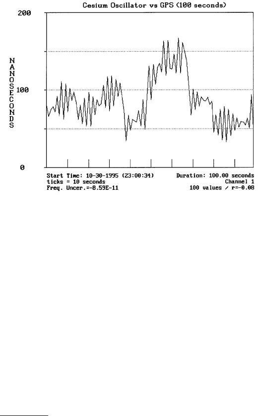
FIGURE 19.8 GPS compared to cesium oscillator over 100 s interval.
phase change, or phase step. A calibration system measures the total amount of phase shift (caused either by the frequency offset of the DUT or a phase step) over a given measurement period.
Figure 19.12 shows a phase comparison between two sinusoidal frequencies. The top sine wave represents a signal from the DUT, and the bottom sine wave represents a signal from the reference. Vertical lines have been drawn through the points where each sine passes through zero. The bottom of the figure shows “bars” that indicate the size of the phase difference between the two signals. If the phase relationship between the signals is changing, the phase difference will either increase or decrease to indicate that the DUT has a frequency offset (high or low) with respect to the reference. Equation 19.1 estimates the frequency offset. In Figure 19.12, both t and T are increasing at the same rate and the phase difference “bars” are getting wider. This indicates that the DUT has a constant frequency offset.
There are several types of calibration systems that can be used to make a phase comparison. The simplest type of system involves directly counting and displaying the frequency output of the DUT with a device called a frequency counter. This method has many applications but is unsuitable for measuring high-performance devices. The DUT is compared to the counter’s timebase (typically a TCXO), and the uncertainty of the system is limited by the performance of the timebase, typically 1 × 10⁻⁸. Some counters allow use of an external timebase, which can improve the results. The biggest limitation is that frequency counters display frequency in hertz and have a limited amount of resolution. Detecting small changes in frequency could take many days or weeks, which makes it difficult or impossible to use this method to adjust a precision oscillator or to measure stability [22]. For this reason, most high-performance calibration systems collect time series data that can be used to estimate both frequency uncertainty and stability. A discussion follows on how phase comparisons are made using two different methods, the time interval method and the dual mixer time difference method [9, 10].
The time interval method uses a device called a time interval counter (TIC) to measure the time interval between two signals. A TIC has inputs for two electrical signals. One signal starts the counter and the
© 1999 by CRC Press LLC
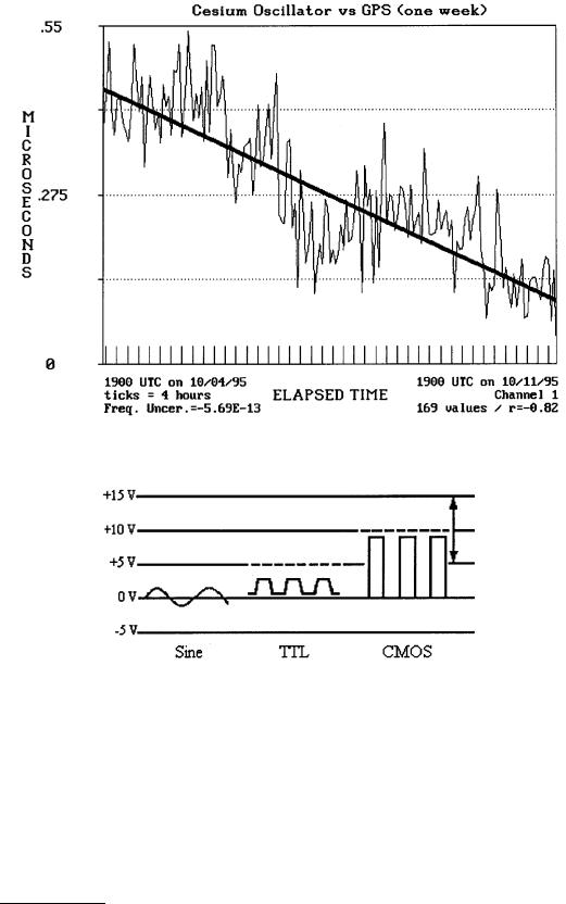
FIGURE 19.9 GPS compared to cesium oscillator over 1 week interval.
FIGURE 19.10 Oscillator outputs.
other signal stops it. If the two signals have the same frequency, the time interval will not change. If the two signals have different frequencies, the time interval will change, although usually very slowly. By looking at the rate of change, one can calibrate the device. It is exactly as if there were two clocks. By reading them each day, one can determine the amount of time one clock gained or lost relative to the other clock. It takes two time interval measurements to produce any useful information. By subtracting the first measurement from the second, one can tell whether time was gained or lost.
TICs differ in specification and design details, but they all contain several basic parts known as the timebase, the main gate, and the counting assembly. The timebase provides evenly spaced pulses used to measure time interval. The timebase is usually an internal quartz oscillator that can often be phase locked to an external reference. It must be stable because timebase errors will directly affect the measurements.
© 1999 by CRC Press LLC
FIGURE 19.11 An oscillating signal.
FIGURE 19.12 Two signals with a changing phase relationship.
The main gate controls the time at which the count begins and ends. Pulses that pass through the gate are routed to the counting assembly, where they are displayed on the TIC’s front panel or read by computer. The counter can then be reset (or armed) to begin another measurement. The stop and start inputs are usually provided with level controls that set the amplitude limit (or trigger level) at which the counter responds to input signals. If the trigger levels are set improperly, a TIC might stop or start when it detects noise or other unwanted signals and produce invalid measurements.
© 1999 by CRC Press LLC

FIGURE 19.13 Measuring time interval.
Figure 19.13 illustrates how a TIC measures the interval between two signals. Input A is the start pulse and Input B is the stop pulse. The TIC begins measuring a time interval when the start signal reaches its trigger level and stops measuring when the stop signal reaches its trigger level. The time interval between the start and stop signals is measured by counting cycles from the timebase. The measurements produced by a TIC are in time units: milliseconds, microseconds, nanoseconds, etc. These measurements assign a value to the phase difference between the reference and the DUT.
The most important specification of a TIC is resolution; that is, the degree to which a measurement can be determined. For example, if a TIC has a resolution of 10 ns, it can produce a reading of 3340 ns or 3350 ns, but not a reading of 3345 ns. Any finer measurement would require more resolution. In simple TIC designs, the resolution is limited to the period of the TIC’s timebase frequency. For example, a TIC with a 10 MHz timebase is limited to a resolution of 100 ns if the unit cannot resolve time intervals smaller than the period of one cycle. To improve this situation, some TIC designers have multiplied the timebase frequency to get more cycles and thus more resolution. For example, multiplying the timebase frequency to 100 MHz makes 10 ns resolution possible, and 1 ns counters have even been built using a 1 GHz timebase. However, a more common way to increase resolution is to detect parts of a timebase cycle through interpolation and not be limited by the number of whole cycles. Interpolation has made 1 ns TICs commonplace, and 10 ps TICs are available [23].
A time interval system is shown in Figure 19.14. This system uses a TIC to measure and record the difference between two signals. Low-frequency start and stop signals must be used (typically 1 Hz). Since oscillators typically produce frequencies like 1, 5, and 10 MHz, the solution is to use a frequency divider to convert them to a lower frequency. A frequency divider could be a stand-alone instrument, a small circuit, or just a single chip. Most divider chips divide by multiples of 10, so it is common to find circuits that divide by a thousand, a million, etc. For example, dividing a 1 MHz signal by 106 produces a 1 Hz signal. Using low-frequency signals reduces the problem of counter overflows and underflows and helps prevent errors that could be made if the start and stop signals are too close together. For example, a TIC might make errors when attempting to measure a time interval of <100 ns.
The time interval method is probably the most common method in use today. It has many advantages, including low cost, simple design, and excellent performance when measuring long-term frequency uncertainty or stability. There are, however, two problems that can limit its performance when measuring short-term stability. The first problem is that after a TIC completes a measurement, the data must be processed before the counter can reset and prepare for the next measurement. During this delay, called dead time, some information is lost. Dead time has become less of a problem with modern TICs where
© 1999 by CRC Press LLC
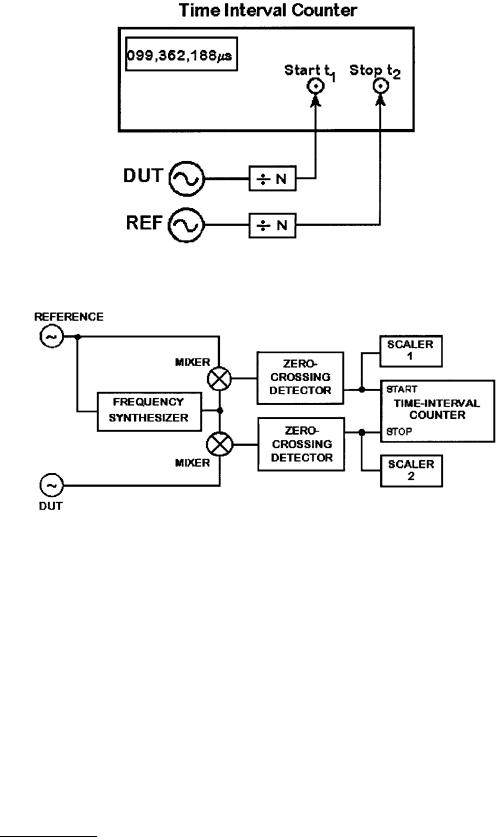
FIGURE 19.14 Time interval system.
FIGURE 19.15 Dual mixer time difference system.
faster hardware and software has reduced the processing time. A more significant problem when measuring short-term stability is that the commonly available frequency dividers are sensitive to temperature changes and are often unstable to ±1 ns. Using more stable dividers adds to the system cost [10, 22].
A more complex system, better suited for measuring short-term stability, uses the Dual Mixer Time Difference (DMTD) method, shown in Figure 19.15. This method uses a frequency synthesizer and two mixers in parallel. The frequency synthesizer is locked to the reference oscillator and produces a frequency lower than the frequency output of the DUT. The synthesized frequency is then heterodyned (or mixed) both with the reference frequency and the output of the DUT to produce two beat frequencies. The beat frequencies are out of phase by an amount proportional to the time difference between the DUT and reference. A zero crossing detector is used to determine the zero crossing of each beat frequency cycle. An event counter (or scaler) accumulates the coarse phase difference between the oscillators by counting the number of whole cycles. A TIC provides the fine-grain resolution needed to count fractional cycles. The resulting system is much better suited for measuring short-term stability than a time interval system. The oscillator, synthesizer, and mixer combination provides the same function as a divider, but the noise is reduced, often to ±5 ps or less.
© 1999 by CRC Press LLC