Charles B. Coulbourn, et. al. "Area Measurement."

Copyright 2000 CRC Press LLC. <http://www.engnetbase.com>.

Area Measurement

Charles B. Coulbourn

One must often measure the area of enclosed regions on plan-size drawings. These areas might be either regular or irregular in shape and describe one of the following:

•Areas enclosed by map contours

•Cross section of the diastolic and systolic volumes of heart cavities

•Farm or forest land shown in aerial photographs

•Cross sections of proposed and existing roads

•Quantities of materials used in clothing manufacture

•Scientific measurements

•Swimming pools

•Quantities of ground cover

Tools for this type of measurement include planimeters, digitizer-computer setups, digitizers with built-in area measuring capability, and grid overlay transparencies.

12.1 Theory

Planimeter

A planimeter is a mechanical integrator that consists of a bar (tracer arm), a measuring wheel with its axis parallel to the bar, and a mechanism that constrains the movement of one end of the bar to a fixed track, Figure 12.1. The opposite end of the bar is equipped with a pointer for tracing the outline of an area. The measuring wheel, Figure 12.2, is calibrated with 1000 or more equal divisions per revolution. Each division equals one count. It accumulates counts, P, according to:

where K = number of counts per revolution of the measuring wheel D = diameter of the measuring wheel

φ = angle between the measuring wheel axis and the direction of travel

s= traced path

©1999 by CRC Press LLC

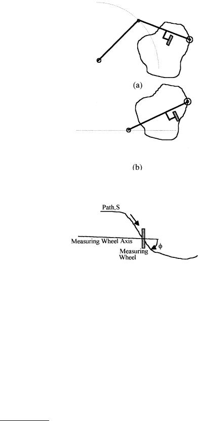
FIGURE 12.1 The constrained end of a polar planimeter (a) follows a circular path; the constrained end of a linear planimeter (b) follows a straight line path.

FIGURE 12.2 The rotation of a measuring wheel is proportional to the product of distance moved and the sine of the angle between the wheel axis and direction of travel.

The size of an area, A, traced is:

where L = length of bar

P = accumulated counts (Equation 12.1)

Figure 12.3 shows how a basic wheel and bar mechanism determines the area of a parallelogram. The traced path is along the sloped line; however, the wheel registers an amount that is a function of the product of the distance traveled and the sine of the angle between the direction of travel and the axis of the measuring wheel (Equation 12.1). This is the altitude of the parallelogram. The product of the altitude (wheel reading converted to distance) and base (bar length) is the area.

Figure 12.4(a) illustrates the operation of a planimeter when the area of a four-sided figure is measured. Figures 12.4(b), (c), (d), and (e) show the initial and final positions of the bar as each side of the figure

© 1999 by CRC Press LLC

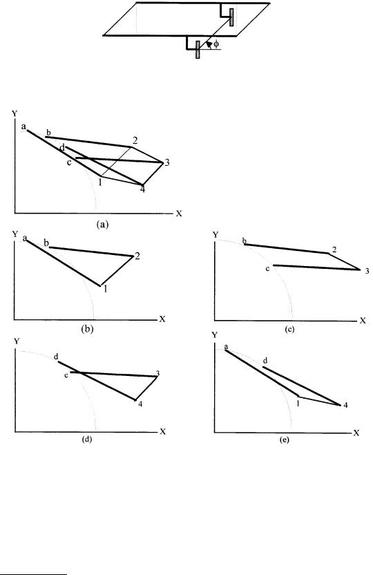
FIGURE 12.3 The area of this parallelogram is proportional to the product of tracer arm length and measuring wheel revolutions.

FIGURE 12.4 This schematic shows a planimeter pointing to each junction of a four-sided figure being traced in (a) and at the ends of each of the segments in (b) through (e). The constrained end of the tracer arm follows a circle.

is traced. Applying the general expression for the area under a curve, A = ∫ f(x)dx for each of these partial areas gives:

© 1999 by CRC Press LLC

where Aa, Ab, Ac, and Ad are the four partial areas.

The total area of the figure is the sum of the four partial areas. Combining the terms of these partial areas and rearranging them so that those defining the area traced by the left end of the bar are in one group, those defining the area traced by the other end of the bar are in a second group, and those remaining are in a third group results in the following:

The first four integrals describe the area traced by the left end of the bar. Since this end runs along an arc, it necessarily encloses an area equal to zero. The final four integral describe the area traced by the right end of the bar. This is the four-sided figure. The remaining eight integrals cancel out since ∫a1 + ∫1a = 0, etc. Thus, the total area equals the area traced by the right end of the bar. Note that the same reasoning applies to figures of any number of sides and of any shape.

Digitizer

A digitizer converts a physical location on a map to digital code representing the (x, y) coordinates of the location. The digital code is normally converted to a standard ASCII or binary format and transmitted to a computer where computations are made to determine such things as area or length. Certain digitizers can also compute areas and lengths without the use of a computer.

Area, A, can be computed using the coordinate pairs that define the area boundary.

A = 12 (y1 + y2 )(x2 - x1) + 12 (y2 + y3 )(x3 - x2 ) + ¼ + 12 (yn −1 + yn )(xn - xn −1)

(12.8)

+ 12 (yn + y1)(x1 - xn )

where x1, x2, x3, etc. = sequentially measured x coordinates along the boundary. y1, y2, y3, etc. = are corresponding y coordinates

© 1999 by CRC Press LLC

All digitized coordinate pairs must be used in the computations since the x intervals of this data are typically unequal.

In Equation 12.8, the final term deserves special consideration because it contains both the first and last coordinate pair of the series. When computations are performed from data stored in a computer, information is available for computing the final term so that no special actions are necessary. However, when the computations are performed by an embedded microprocessor with limited memory, normally each term is computed as the coordinates are read. In this case, one of two actions must be taken. First, the first coordinate pair is saved and then, once the measurement has been completed, a key is pressed to initiate computation of the final term. This is called “closing the area.” Second, if the first coordinate pair is not saved, to prevent an error the final point digitized must coincide with the first point digitized so that xn = x1, yn = y1 and the final term is zero.

Popular types of digitizers in use today are tablets, sonic digitizers, and arm digitizers. Probably the most popular type is the tablet.

Tablet Digitizer

Tablet digitizers consist of a pointer and a work surface containing embedded wires configured as a grid. The horizontal wires are parallel and spaced by about 12 mm. The vertical wires are also parallel and spaced the same. Different sensing techniques are used to locate the pointer position relative to the grid wires.

One sensing technique employs grid wires made from magnetostrictive material that has the property of changing shape very rapidly when subjected to a magnetic field. Each set of grid wires, the horizontal and vertical, is independently energized by a send wire that lies perpendicular to that set of wires [1]. A pulse transmitted over the send wire has a magnetic field that changes the shape of each magnetostrictive wire, causing a strain wave to propagate down the wire. Coincidentally, the pulse starts a counter. A coil in the pointer senses the strain wave and sends a signal to stop the counter. The counter reading is thus proportional to the propagation time of the strain wave. The product of the propagation time and velocity of the strain wave equals the physical distance between send line and pointer detector. The velocity of the strain waves is slow enough so that any errors in time measurement can be made acceptable.

A second sensing technique uses a grid made of conductive wires and a pointer that emits a signal on the order of 57.6 kHz [2]. The vertical grid wires are sensed to determine the amplitude distribution of signal induced in each wire. The point of maximum signal strength determines the location of the pointer along the horizontal axis. The horizontal grid wires are likewise sensed to find the point of maximum signal strength that determines the pointer location along the vertical axis. Coupling between the pointer and grid can be by either electromagnetic or by electrostatic means [3].

Signals can also be applied to the grid wires and the pointer used as a receiver. In this case, the signal to each grid wire must be coded or else applied sequentially, first to one set of grid wires and then to the other. Amplitude profiles of the signals received by the pointer are determined to locate the pointer along each axis.

Sonic Digitizers

Sonic digitizers consist of a pointer and two or more microphones. The pointer, used to identify the point to be digitized, typically contains a spark gap that periodically emits a pulse of sonic energy [4]. The microphones in certain cases are mounted in a bar that is located along the top of the drawing area. In other cases, they are mounted in an L frame and located along the top and one side of the drawing area.

The microphones receive the sonic pulse emitted by the pointer. The time taken for the pulse to travel from the transmitter to each receiver is measured and the slant distance computed from the product of this elapsed time and the sonic velocity. The x and y coordinates of the pointer are computed from the slant ranges and the locations of the microphones.

Ambiguities exist since a single set of slant ranges describe two points; however, the ambiguities can be resolved either by using additional microphones or by ensuring that the ambiguous points are outside the work area. With the microphones aligned along the top of the work area, the ambiguous points are

© 1999 by CRC Press LLC