Micro-Cap v7.1.6 / RM

when their FREQ attribute is specified, resistors, capacitors, inductors, and NFV and NFI function sources. Z transform and Laplace sources use the complex frequency variable S ( j*2*PI*frequency ) in their transfer function, so their transfer function must change with frequency during the run.

For curve sources, the small signal model is simply an AC voltage or current source. The AC value of the source is determined from the parameter line for SPICE components and from the attribute value for schematic components.

SPICE V or I sources:

The AC magnitude value is specified as a part of the device parameter. For example, a source with the value attribute "DC 5.5 AC 2.0" has an AC magnitude of 2.0 volts.

Pulse and sine sources:

These sources have their AC magnitude fixed at 1.0 volt.

User sources: User sources provide a signal comprised of the real and imaginary parts specified in their files.

Function sources: These sources create an AC signal only if a FREQ expression is specified.

Because AC analysis is linear, it doesn't matter whether the AC amplitude of a single input source is 1 volt or 500 volts. If you are interested in relative gain from one part of the circuit to another, then plot V(OUT)/V(IN). This ratio will be the same regardless of the value of V(IN). If V(IN) is 1, then it is not necessary to plot ratios, since V(OUT)/V(IN) = V(OUT)/1 = V(OUT). If there is more than one input source with a nonzero AC value, then you can't meaningfully look at gains from one of the source nodes to another node.

The basic sequence for AC analysis is this:

1.Optionally calculate the DC operating point.

2.Compose the linear equivalent AC model for every device.

3.Construct a set of linearized circuit equations.

4.Set frequency to fmin.

5.Solve for all voltages and currents in the linearized model.

6.Plot or print requested variables.

7.Increment frequency.

8.If frequency exceeds fmax, quit, else go to step 5.

127

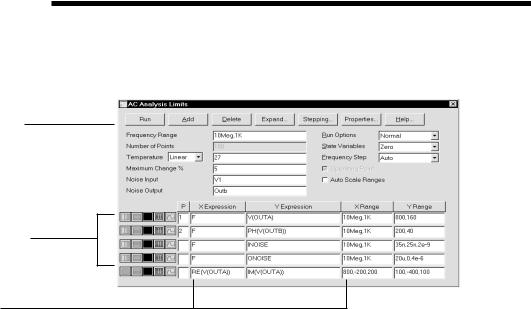
The AC Analysis Limits dialog box

The Analysis Limits dialog box is divided into five principal areas: the Command buttons, Numeric limits, Curve options, Expressions, and Options.

Command buttons

Curve options

Expressions

Figure 7-1 The Analysis Limits dialog box

The command buttons are located just above the Numeric limits.

Run: This command starts the analysis run. Clicking the Tool bar Run button or pressing F2 will also start the run.

Add: This command adds another Curve options field and Expression field line after the line containing the cursor. The scroll bar to the right of the Expression field scrolls the curve rows when needed.

Delete: This command deletes the Curve option field and Expression field line where the text cursor is.

Expand: This command expands the working area for the text field where the text cursor currently is. A dialog box is provided for editing or viewing. To use the feature, click in an expression field, then click the Expand button.

Stepping: This command calls up the Stepping dialog box. Stepping is reviewed in a separate chapter.

128 Chapter 7: AC Analysis

Properties: This command invokes the Properties dialog box which lets you control the analysis plot window and the way curves are displayed.

Help: This command calls up the Help system which provides information by index and topic.

The definition of each item in the Numeric limits field is as follows:

•Frequency Range: This field controls the frequency range for the analysis. The syntax is <Highest Frequency> [, <Lowest Frequency>]. If <Lowest Frequency> is unspecified, the program calculates a single data point at <Highest Frequency>.

•Number of Points: This determines the number of data points printed in the Numeric Output window. It also determines the number of data points actually calculated if Linear or Log stepping is used. If the Auto Step method is selected, the number of points actually calculated is controlled by the <Maximum change %> value. If Auto is selected, interpolation is used to produce the specified number of points. The default value is 51. This number is usually set to an odd value to produce an even print interval.

For the Linear method, the frequency step and the print interval are: (<Highest Frequency> - <Lowest Frequency>)/(<Number of points> - 1) For the Log method, the frequency step is:

(<Highest Frequency> / <Lowest Frequency>)1/(<Number of points> - 1)

• Temperature: This field controls the temperature of the run. If the Temperature list box shows Linear the format is:

<high> [ , <low> [ , <step> ] ]

The default value of <low> is <high>, and the default value of <step> is <high> - <low>.

If the Temperature list box shows List the format is: <t1> [ , <t2> [ , <t3> ] [ ,...]]

where t1, t2,.. are individual values of temperature.

129

mon expressions are F (frequency), db(v(1)) (voltage in decibels at node 1), and re(v(1)) (real voltage at node 1). Note that while the expressions are evaluated as complex quantities, only the magnitude of the Y expression vs. the magnitude of the X expression is plotted. If you plot the expression V(3)/V(2), MC7 evaluates the expression as a complex quantity, then plots the magnitude of the final result. It is not possible to plot a complex quantity directly versus frequency. You can plot the imaginary part of an expression versus its real part (Nyquist plot), or you can plot the magnitude, real, or imaginary parts versus frequency (Bode plot).

The scale ranges specify the scales to use when plotting the X and Y expressions. The range format is:

<high> [,<low>] [,<grid spacing>] [,<bold grid spacing>]

<low> defaults to zero. [,<grid spacing>] sets the spacing between grids. [,<bold grid spacing>] sets the spacing between bold grids. Placing "AUTO" in the X or Y scale range calculates its range automatically. The Auto Scale Ranges option calculates scales for all ranges during the simulation run and updates the X and Y Range fields. The Auto Scale (F6) command immediately scales all curves, without changing the range values, letting you restore them with CTRL + HOME if desired. Note that <grid spacing> and <bold grid spacing> are used only on linear scales. Logarithmic scales use a natural grid spacing of 1/10 the major grid values and bold is not used. The Auto Scale command uses the Preferences / Auto Scale Grids value to set the grid spacing.

Clicking the right mouse button in the Y expression field invokes the Variables list. It lets you select variables, constants, functions, and operators, or expand the field to allow editing long expressions. Clicking the right mouse button in the other fields invokes a simpler menu showing suitable choices.

The Options group includes:

•Run Options

•Normal: This runs the simulation without saving it to disk.

•Save: This runs the simulation and saves it to disk.

•Retrieve: This loads a previously saved simulation and plots and prints it as if it were a new run.

•State Variables: These options determine what happens to the time

131

domain state variables (DC voltages, currents, and digital states) prior to the optional operating point.

•Zero: This sets the state variable initial values (node voltages, inductor currents, digital states) to zero or X.

•Read: This reads a previously saved set of state variables and uses them as the initial values for the run.

•Leave: This leaves the current values of state variables alone. They retain their last values. If this is the first run, they are zero. If you have just run an analysis without returning to the Schematic editor, they are the values from that run.

•Frequency step

•Auto: This method uses the first plot of the first group as a pilot plot. If, from one frequency point to another, the plot has a vertical change of greater than Maximum change % of full scale, the frequency step is reduced, otherwise it is increased. Maximum change % is the value from the fourth numeric field of the AC Analysis Limits dialog box. Auto is the standard.

•Linear: This method produces a frequency step such that, with a linear horizontal scale, the data points are equidistant horizontally.

•Log: This method produces a frequency step such that with a log horizontal scale, the data points are equidistant horizontally.

•List: This method uses a comma-delimited list of frequency points from the Frequency Range, as in 1E8, 1E7, 5E6.

•Operating Point: This calculates a DC operating point, changing the timedomain state variables as a result. If an operating point is not done, the time domain variables are those resulting from the initialization step (zero, leave, or read). The linearization is done using the state variables after this optional operating point. In a nonlinear circuit where no operating point is done, the validity of the small-signal analysis depends upon the accuracy of the state variables read from disk, edited manually, or enforced by device initial values or .IC statements.

•Auto Scale Ranges: This sets all ranges to Auto every time a simulation is run. If disabled, the values from the range fields are used.

132 Chapter 7: AC Analysis

The AC menu

Run: (F2) This starts the analysis run.

Limits: (F9) This accesses the Analysis Limits dialog box.

Stepping: (F11) This accesses the Stepping dialog box.

Optimize: (CTRL + F11) This accesses the Optimize dialog box.

Analysis Window: (F4) This command displays the analysis plot.

Watch: (CTRL + W) This displays the Watch window where you define expressions or variables to watch during a breakpoint invocation.

Breakpoints: (ALT + F9) This accesses the Breakpoints dialog box. Breakpoints are Boolean expressions that define when the program will enter single-step mode so that you can watch specific variables or expressions. Typical breakpoints are F>=10Meg AND F<=110Meg, or V(OUT)>2.

3D Windows: This lets you add or delete a 3D plot window. It is enabled only if more than one run is done.

Performance Windows: This lets you add or delete a performance plot window. It is enabled only if there is more than one run.

Numeric Output: (F5) This shows the Numeric Output window.

State Variables editor: (F12) This accesses the State Variables editor.

DSP Parameters: This opens the DSP dialog box. It lets you specify the frequency window lower and upper limits and the number of sample points to use for the DSP functions. See Chapter 24, "Fourier Analysis and Digital Signal Processing", for more details on DSP functions.

Reduce Data Points: This item invokes the Data Point Reduction dialog box. It lets you delete every n'th data point. This is useful when you use very small time steps to obtain very high accuracy, but do not need all of the data points produced. Once deleted, the data points cannot be recovered.

Exit Analysis: (F3) This exits the analysis.

133

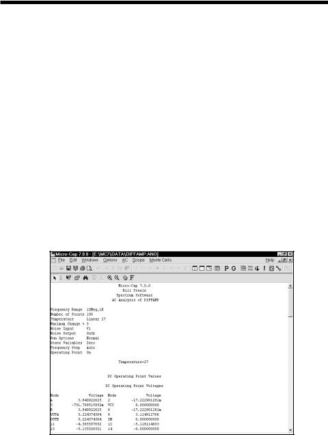
Numeric output

Numeric output may be obtained for the X and Y expressions of each curve by clicking the button in the curve row. Numeric output includes:

Analysis Limits Summary: This is a printout of the main analysis limits from the Analysis Limits, Stepping, and Monte Carlo dialog boxes.

Operating point information: This is a printout of the DC operating point values for each device in the circuit. It includes a selection of device currents, voltages, conductances, and capacitances.

Curve tables: These are tabular printouts of the value of each X and Y expression of selected curves. Duplicated X expressions (like F for frequency) are eliminated.

Output is saved to the text file CIRCUITNAME.ANO and printed to the window, which is accessible after the run by clicking on the button. Here is a typical result.

Figure 7-2 Numeric output

134 Chapter 7: AC Analysis

Noise

MC7, like SPICE, models three types of noise:

•Thermal noise

•Shot noise

•Flicker noise

Thermal noise, produced by the random thermal motion of electrons, is always associated with resistance. Discrete resistors and the parasitic resistance of active devices contribute thermal noise.

Shot noise is caused by a random variation in current, usually due to recombination and injection. Normally, shot noise is associated with the dependent current sources used in the active device models. All semiconductor devices generate shot noise.

Flicker noise originates from a variety of sources. In BJTs, the source is normally contamination traps and other crystal defects that randomly release their captured carriers.

Noise analysis measures the contribution from all of these noise sources as seen at the input and output. Output noise is calculated across the output node(s) specified in the Noise Output field. To plot or print it, specify 'ONOISE' as the Y expression. Similarly, input noise is calculated across the same output nodes, but is divided by the gain from the input node to the output node. To plot or print input noise, specify "INOISE" as the Y expression.

Because the network equations are structured differently for noise, it is not possible to simultaneously plot noise variables and other types of variables such as voltage and current. If you attempt to plot both noise and other variables, the program will issue an error message.

Because noise is an essentially random process, there is no phase information. Noise is defined as an RMS quantity so the phase (PH) and group delay (GD) operators should not be used.

Noise is measured in units of Volts / Hz1/2.

135

AC analysis tips

Here are some useful things to remember for AC analysis:

Unexpected output when bypassing the operating point:

If your circuit is producing strange results and you are not doing an operating point, make sure that the initial conditions you've supplied are correct. You must supply all node voltages, inductor currents, and digital states if you skip the operating point in order to get meaningful results.

Zero output:

If your circuit is producing zero voltages and currents it is probably because the sources are absent or have zero AC magnitudes. Only the PULSE and SIN sources have a nonzero 1.0 default AC magnitude. The User source supplies what its file specifies. Function sources generate an AC excitation equal to the value of their FREQ expression, if any. The other sources either have no AC magnitude at all or else have a 0.0 volt default AC magnitude.

Simultaneous Auto Frequency step and Auto Scale:

If you select both Auto frequency stepping and Auto Scale, the first plot will probably be coarse. Auto frequency stepping uses the plot scale employed during the run to make dynamic decisions about a suitable frequency step. If Auto Scale is in effect, the plot scale employed during the run is preset to a very coarse scale. The frequency steps are not referenced to the actual range of the curve, since it is only known after the run. The solution is to make two runs, and turn off the Auto Scale option after the first run. The second run will have the benefit of knowing the true range of the curve

and will produce a smoother plot.

Flat curves:

If your circuit is a very narrow band reject filter and your gain plot is flat, it is probably because the frequency step control is not sampling in the notch. This can happen when the sweep starts at a frequency far to the left of the notch. Since the plot is very flat, the frequency step is quickly increased to the maximum. By the time the frequency nears the notch, the step exceeds the notch width and the sweep jumps over the notch. This is like a car moving so fast that is doesn't notice a narrow pothole that would have been apparent at a lower speed. The solution is to set the fmin much nearer the expected notch, or use one of the fixed frequency step methods. If you use a fixed step, make sure the frequency step is smaller than the notch. This can be

136 Chapter 7: AC Analysis