

Micro-Cap v7.1.6 / RM
.PDFDelay Filters:
Gain
This is the low frequency gain in dB.
Delay
This is the filter delay in seconds.
187

How the passive filter designer works
The passive filter design function operates in a manner similar to the active filter function. It is selected from the Design menu. Like its active filter counterpart, it lets you select the filter type, specifications, response, and circuit implementation, then creates the required filter circuit.
The basic filter types include:
•Low pass
•High pass
•Bandpass
•Notch
The filter responses include:
•Butterworth
•Chebyshev
The implementations are of two types:
•Standard
•Dual
188 Chapter 12: Active Filter Designer
The Passive Filter dialog box
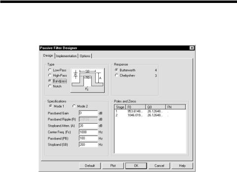
The passive filter design function is accessed from the Design menu. Selecting it invokes the following dialog box:
Figure 12-9 The passive filter design panel
This dialog box has three main panels, accessible by clicking on a named tab.
Design
This panel lets you pick the filter type, specifications, and the response characteristic. Each time you change one of these selections, the number of stages, the pole location, and the Q value change as shown in the Poles and Zeros display. You can edit the F0 (pole frequency) and Q0 (Q value) values to change the shape of the response.
Implementation
This panel lets you make the implementation decisions, including which circuit to use, whether to use exact passive component values or to select them from specified lists, whether to scale the values or not, and the source and load resistances.
Options
In this panel you choose the number of digits of precision to be used in the component values, what to plot, whether to create a macro or a circuit, and whether to use an existing circuit or a new one.
189
Design Panel
The main panel contains three sections:
Type: This section lets you select one of the filter types:
•Low pass
•High pass
•Bandpass
•Notch
Response: This section lets you select the mathematical approximation to the ideal filter.
•Butterworth
•Chebyshev
Different responses provide different design trade-offs. Butterworth filters require much more circuitry for a given specification, but have a flatter time delay response. Chebyshev responses require fewer stages, but have a more pronounced time delay variation. The number of stages to implement the current design is shown to the right of each response.
Specifications: This is where you enter the numerical specifications of the filter. There are two ways to specify a filter, Mode 1 and Mode 2. In Mode 1, you specify the functional characteristics of the filter, like passband gain, cutoff frequency, stop frequency, and attenuation. You specify what you want and the program figures out the number of stages required to achieve it, using the specified response approximation. Mode 2, on the other hand, lets you directly specify the main design values and the number of stages.
Poles and Zeros: This section shows the numeric values of the poles and Qs of the response polynomial. It essentially shows the mathematical design of the filter. When you make a change to the Type, Response, or Specifications fields, the program redesigns the polynomial coefficients and updates the numbers in this section. If the Plot button has been clicked, the program also redraws the response plot. It may be a Bode plot with gain, phase, and group delay show, or it may be just a delay plot, depending upon the selections in the Options panel.
The plot is idealized because it is based on a standard polynomial formula for the selected response and the calculated or edited F0 and Q0 values. Its plot can only be achieved exactly with perfect components. The actual filter, made from real
190 Chapter 12: Active Filter Designer
components, may behave differently. When the circuit is completed, you can run an analysis and see how it behaves. The actual circuit can be constructed from a finite list of standard inductors and capacitors. Approximate component values can have a big effect on the response curves.
You can edit the values, to see their effect on the plot. You can even create your filter with modified values. Though this will not produce an ideal filter, the circuit created will approximate the plot shown. Note that editing any item in the Type, Response, or Specifications areas will cause the program to recalculate the values, overwriting your edits.
The exact form of the approximating polynomials for each stage is shown below. Note that U is the complex frequency variable S, normalized to the specified FC.
Definitions
Symbol Definition
F |
Frequency variable |
|
S |
J*2*PI*F |
Complex frequency |
U |
S / (2*PI*FC) = J*F/FC |
Normalized complex frequency |
F0 |
Pole location in Hz |
|
Q0 |
Q value |
|
FC |
Stopband frequency for low-pass filters. Passband frequency for |
|
|
high-pass filters. Center frequency for bandpass and notch filters. |
|
|
Note that the specified center frequency may be changed slightly by |
|
|
the program to produce a symmetrical band pass/reject region. The |
|
|
adjusted F0 can be seen in the define statement. For example, a |
|
|
Butterworth bandpass filter using the default center frequency of |
|
|
1000, and bandwidth of 100, is actually designed with a center |
|
|
frequency of 998.75 Hz. |
|
W0 |
F0/FC |
Normalized pole frequency |
191
Low Pass Transfer Functions
Butterworth |
F(U) = 1 / (U2 +U/Q0 + 1) |
Chebyshev |
F(U) = 1 / (U2 +U*W0/Q0 + W02) |
High Pass Transfer Functions |
|
Butterworth |
F(U) = U2 / (U2 +U/Q0 + 1) |
Chebyshev |
F(U) = U2 / (U2 +U/(W0*Q0) + 1/W02) |
Bandpass Transfer Functions |
|
Butterworth |
F(U) = U / (U2 +U/(W0*Q0) + 1/W02) |
Chebyshev |
F(U) = U / (U2 +U/(W0*Q0) + 1/W02) |
Notch Transfer Functions |
|
Butterworth |
F(U) = (U2+1) / (U2 +U/(W0*Q0) + 1/W02) |
Chebyshev |
F(U) = (U2+1) / (U2 +U/(W0*Q0) + 1/W02) |
192 Chapter 12: Active Filter Designer
Implementation Panel
This panel lets you decide how to build or implement the filter design.
It has several major sections:
Circuit: This section lets you specify whether to use the standard LC passive circuit, or its dual circuit.
Resistor Values: This section lets you specify whether to use exact values or to select them from a specified file. These choices are used only for the source and load resistors.
Capacitor Values: This section lets you specify whether to use exact capacitor values or to select them from a specified file.
Inductor Values: This section lets you specify whether to use exact inductor values or to select them from a specified file.
Impedance Scale Factor: This option lets you specify a scale factor to apply to all passive component values. The factor multiplies all resistor and inductor values and divides all capacitor values. It does not change the shape of the response curve, but is used to shift component values to more suitable or practical values.
Source/Load Resistor: This option lets you specify the desired source and load resistor value. If the Exact option is selected, this value, after multiplication by the impedance scale factor, will be used for the source and load resistors in the final circuit. If the Exact option is not checked and a resistor file (*.res) is selected, the value in the resistor file nearest the desired value will be used instead.
Options Panel
The options panel has the same content and use as in the active filter design function. It lets you set component value and polynomial numeric format, determine what to plot and how to plot it, whether to create a circuit or a macro, whether to place the filter in the current or a new circuit, and whether to add a title and polynomial text.
193
194 Chapter 12: Active Filter Designer

Chapter 13 |
Scope |
What's in this chapter
Scope is a term for the collection of tools for displaying, analyzing, and annotating the analysis plot and its curves. Available in transient, AC, and DC analysis, it lets you expand, contract, pan, and manipulate curves, and display their numeric values. Cursors are available with commands to locate local curve peaks, valleys, maxima, minima, slopes, inflection points, and specific values. Tags, text, and graphics are available to annotate and document the plot.
Features new in Micro-Cap 7
•Label Data Points command.
•Label Branches command.
•Mouse or Go To Branch command to select individual branches.
•Top and Bottom to find branch extremes.
•Even Decimal Values Cursor Positioning Mode.
•Incremental auto-ranging.
•New Grid Type (+).
•New range format <high> [,<low>] [,<grid spacing>] [,<bold spacing>]
•Plot Grids Quantity, Width, and Pattern Control.
•Thumb Nail Plot.
195
Analysis plot modes
After an AC, DC, or transient analysis is over, there are several modes for reviewing, analyzing, and annotating the analysis plot.
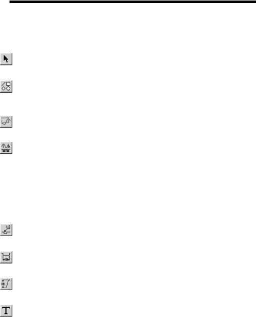
•Select: (CTRL + E) In this mode, the left mouse button is used to select text, tags, and graphic objects for moving and editing.
•Graphics: Clicking on this button lets you select a graphic object (line, ellipse, rectangle, diamond, arc, pie, or polygon) for placement on the plot. Once the object has been selected you drag the mouse to create the object.
•Scale: (F7) In this mode, you can drag the left mouse button to define a plot region tomagnify.
•Cursor: (F8) In this mode, the display shows the value of each curve at each of two numeric cursors. The left mouse button controls the left cursor and the right button controls the right cursor. The left cursor is initially placed on the first data point. The right cursor is initially placed on the last data point. The LEFT ARROW or RIGHT ARROW keys move the left cursor (or right cursor if SHIFT is also pressed) to a point on the selected curve. Depending on the cursor positioning mode, the point may be the next local peak or valley, global high or low, inflection point, or simply the next data point.
•Point Tag: In this mode, the left mouse button is used to tag a data point with its numeric (X,Y) value. The tag will snap to the nearest data point.
•Horizontal Tag: In this mode, the left mouse button is used to drag between two data points to measure the horizontal delta.
•Vertical Tag: In this mode, the left mouse button is used to drag between two data points to measure the vertical delta.
•Text: (CTRL + T ) This mode lets you place text on an analysis plot. You can place relative or absolute text. Relative text maintains its position relative to the curve when the plot scale is changed. Absolute text maintains its position relative to the plot frame. You can also control text border and fill colors, orientation, font, style, size, and effects.
196 Chapter 13: Scope