

Micro-Cap v7.1.6 / RM
.PDFexpand the field to allow editing long expressions. Clicking the right mouse button in the other fields invokes a simpler menu showing suitable choices.
The X Range and Y Range fields specify the numeric scales to be used when plotting the X and Y expressions.
|
The format is: |
|
|
<high> [,<low>] [,<grid spacing>] [,<bold grid spacing>] |
|
|
<low> defaults to zero. [,<grid spacing>] sets the spacing between grids. |
|
|
[,<bold grid spacing>] sets the spacing between bold grids. Placing "AUTO" in |
|
|
the X or Y range calculates the range automatically. The Auto Scale Ranges option |
|
|
calculates scales for all ranges during the simulation run and updates the X and Y |
|
|
Range fields. The Auto Scale (F6) command immediately scales all curves, without |
|
|
changing the range values, letting you restore them with CTRL + HOME if de- |
|
|
sired. Note that <grid spacing> and <bold grid spacing> are used only on linear |
|
|
scales. Logarithmic scales use a natural grid spacing of 1/10 the major grid values |
|
|
and bold is not used. The Auto Scale command uses the Preferences / Auto Scale |
|
|
Grids value to set the grid spacing. |
|
|
These options include the following: |
|
Transient |
||
• Run Options |
||
options |
||
|
• Normal: This runs the simulation without saving it. |
|
|
• Save: This runs the simulation and saves it to disk, using the same |
|
|
format as in Probe. The file name is NAME.TSA. |
|
|
• Retrieve: This loads a previously saved simulation and plots and prints |
|
|
it as if it were a new run. The file name is NAME.TSA. |
|
|
• State Variables |
|
|
These options determine the state variables at the start of the next run. |
|
|
• Zero: This sets the state variable initial values (node voltages, inductor |
|
|
currents, digital states) to zero or X. |
|
|
• Read: This reads a previously saved set of state variables and uses |
|
|
them as the initial values for the run. |
117
• Leave: This leaves the current values of state variables alone. They retain their last values. If this is the first run, they are zero. If you have just run an analysis without returning to the Schematic editor, they are the values at the end of the run. If the run was an operating point only run, the values are the DC operating point.
•Operating Point: This calculates a DC operating point. It uses the initial state variables as a starting point and calculates a new set that represents the DC steady state response of the circuit to the T=0 values of all sources.
•Operating Point Only: This calculates a DC operating point only. No transient run is made. The state variables are left with their final operating point values.
•Auto Scale Ranges: This sets the X and Y range to AUTO for each new analysis run. If it is not enabled, the existing scale values from the X and Y Range fields are used.
The Run, State Variables, and Analysis options affect the simulation results. To see the effect of changes of these options you must do a run by clicking on the Run command button or pressing F2.
118 Chapter 6: Transient Analysis
The Transient menu
Run: (F2) This starts the analysis run.
Limits: (F9) This accesses the Analysis Limits dialog box.
Stepping: (F11) This accesses the Stepping dialog box.
Optimize: (CTRL + F11) This accesses the Optimize dialog box.
Analysis Window: (F4) This command displays the analysis plot.
Watch: (CTRL + W) This displays the Watch window where you define expressions or variables to watch during a breakpoint invocation.
Breakpoints: (ALT + F9) This accesses the Breakpoints dialog box. Breakpoints are Boolean expressions that define when the program will enter single-step mode so that you can watch specific variables or expressions. Typical breakpoints are T>=100ns AND T<=10ns, or V(OUT)>5.5.
3D Windows: This lets you add or delete a 3D plot window. It is enabled only if more than one run is done.
Performance Windows: This lets you add or delete a performance plot window. It is enabled only if there is more than one run.
Numeric Output: (F5) This shows the Numeric Output window.
State Variables editor: (F12) This accesses the State Variables editor.
DSP Parameters: This opens the DSP dialog box. It lets you specify the time window lower and upper limits and the number of sample points to use for the DSP functions. See Chapter 24, "Fourier Analysis and Digital Signal Processing", for more details on DSP functions.
Reduce Data Points: This item invokes the Data Point Reduction dialog box. It lets you delete every n'th data point. This is useful when you use very small time steps to obtain very high accuracy, but do not need all of the data points produced. Once deleted, the data points cannot be recovered.
Exit Analysis: (F3) This exits the analysis.
119

Initialization
State variables define the state or condition of the mathematical system that represents the circuit at any instant. These variables must be initialized to some value prior to starting the analysis run. Here is how MC7 does the initialization:
Setup initialization:
When you first select a transient, AC, or DC analysis, all state variables are set to zero and all digital levels to X. This is called the setup initialization.
Run initialization:
Each new run evokes the run initialization based upon the State Variables option from the Analysis Limits dialog box. This includes every run, whether initiated by pressing F2, clicking on the Run button, stepping parameters, using Monte Carlo, or stepping temperature. There are three choices:
Zero: The analog state variables, node voltages, and inductor currents are set to 0. Digital levels are set to X, or in the case of flip-flop Q and QB outputs, set to '0', '1', or 'X' depending upon the value of the global value DIGINITSTATE. This value is defined in the Global Settings dialog box. This is the only option in DC analysis.
Read: MC7 reads the variables from the file CIRCUITNAME.TOP. The file itself is created by the State Variables editor Write command.
Leave: MC7 does nothing to the state variables. It simply leaves them alone. There are three possibilities:
First run: If the variables have not been edited with the State Variables editor, they still retain the setup initialization values.
Later run: If the variables have not been edited with the State Variables editor, they retain the ending values from the last run.
Edited: If the variables have been edited with the State
Variables editor, they are the values shown in the editor.
After the State Variables option has been processed, .IC statements are processed. Device IC statements, such as those for inductor current and capacitor voltage, override .IC statements if they are in conflict.
120 Chapter 6: Transient Analysis

Note that .IC statements specify values that persist throughout the initial bias point calculation.
They are more resilient than simple initial values which can (and usually do) change after the first iteration of the bias point. This may be good or bad depending upon what you are trying to achieve.
Using these initial values, an optional operating point calculation may be done and the state variables may change. If no operating point is done, the state variables are left unchanged from the initialization procedure. If an operating point only is done, the ending state variable values are equal to the DC operating point values.
Using the P key
During a simulation run, the value of the expressions for each curve can be seen by pressing the 'P' key. This key toggles the printing of the numeric values on the analysis plot adjacent to the expressions. This is a convenient way to check the course of a new, lengthy simulation when the initial plot scales are unknown. This feature may significantly slow the simulation, so only use it to "peek" at the numeric results, then toggle it off with the 'P' key.
121
The State Variables editor
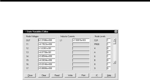
The State Variables editor is for reviewing or editing state variables. It looks likes this:
Figure 6-2 The State Variables editor
The editor displays node voltages, inductor currents, and digital node levels. The scroll bars may be used to review values not visible on the display. Any value may be edited.
The command buttons function as follows:
•Close: This exits the dialog box.
•Clear: This immediately sets all analog values to zero. Digital node levels are set to 'X'.
•Read: This immediately reads a new set of values from a disk file, after prompting for a file name.
•Write: This immediately writes the displayed values to a disk file using a user-supplied file name. This file is created for use when the Analysis Limits State Variables Read option is selected. The Read option uses the values stored in this file at the Run initialization stage.
•Print: This copies the values to a text file called CIRCUITNAME.SVV.
•.IC:This command translates the existing state variables into .IC statements and saves them in the circuit's text area. The following translations are made:
122 Chapter 6: Transient Analysis
State variable |
IC statement |
Node voltage |
.IC V(Node name) = Node voltage |
Inductor current |
.IC I(Inductor name) = Inductor current |
Digital node state |
.IC D(Digital node name) = Digital node state |
The purpose of this command is to provide a handy way to create .IC statements, which some prefer as a means of initializing state variables.
It is important to note that the clear and read commands, and all manual edits result in immediate changes, as opposed to the delayed changes made by the Analysis Limits options. The Zero, Read, and Leave options from the Analysis Limits dialog box affect the values at the start of the simulation (Run initialization).
• Help: This accesses help topics for the State Variables editor.
123
Numeric output
Numeric output may be obtained for each curve by clicking the Numeric Output button  in the curve row. Numeric output is of several types:
Analysis Limits Summary: This is a printout of the main analysis limits from the Analysis Limits, Stepping, and Monte Carlo dialog boxes.
Operating point information: This is a printout of the DC operating point values for each device in the circuit. It includes a selection of device currents, voltages, conductances, and capacitances.
Curve tables: This is a tabular printout of the value of each X and Y expression of each selected curve. The values are interpolated from the actual data points. The Number of Points value from the Analysis Limits dialog box determines the number of points printed in the table.
Digital warnings: These include digital hazard and constraint violations.
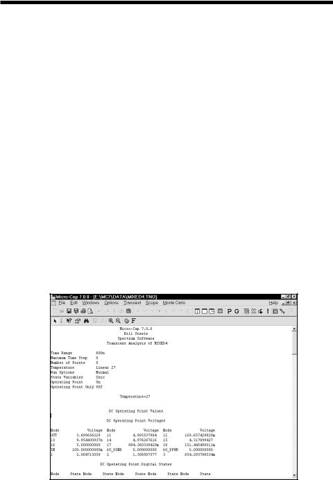
Output is saved in the file CIRCUITNAME.TNO and printed to the Numeric Output window, which is accessible after the run by clicking on the  button. Here is a typical output window.
Figure 6-3 Numeric output
124 Chapter 6: Transient Analysis

Chapter 7 |
AC Analysis |
What's in this chapter
This chapter describes the AC analysis routines. AC analysis is a linear, small signal analysis. Before the main AC analysis is run, linearized small signal models are created for nonlinear components based upon the operating point bias.
Features new in Micro-Cap 7
•Smith charts
•Polar plots
•Optimizer
•Watch window
•Breakpoints window
•Range format <high> [,<low>] [,<grid spacing>] [,<bold spacing>]
125

What happens in AC analysis
AC analysis is a type of small-signal or linear analysis. This means that all circuit variables are assumed to be linearly related. Double one voltage, and you double any related quantities. When you plot or print V(1) you are seeing the small-signal linear voltage between node 1 and the ground node.
Using a small-signal model of each device in the circuit, MC7 constructs a set of linear network equations and solves for every voltage and current in the circuit over the specified frequency range. The program obtains the small-signal models by linearizing the devices about the state variable values. These are usually the result of an operating point calculation, but may also result from a read, from edits in the State Variables editor, or may simply be left over from the last run.
Linearizing means replacing a device's nonlinear model with a simple constant that expresses a linear relationship between the terminal voltages and currents of the device. The linear model is assumed to hold for small signal changes about the point at which the linearization takes place, the DC operating point. Digital parts are treated as open circuits during the linearization process. For linear resistors, capacitors, and inductors, the linearized AC value is the same as the constant time-domain value. For nonlinear passive components whose value changes with bias, the linearized AC value is the time-domain resistance, capacitance, or inductance computed at the operating point. This means that in a resistor with a value expression like 1+2*V(10), the V(10) refers to the time-domain V(10), not the AC small signal V(10). If the operating point calculation produces a DC value of 2.0 volts for V(10), then the value of this resistor during AC analysis will be 1+2*2 = 5 Ohms. During the small-signal AC analysis, the resistance, capacitance, or inductance does not change. There is an exception to this rule however.
If the component's FREQ attribute is specified, then the FREQ expression is the AC resistance, capacitance, or inductance, and is allowed to be a function of frequency. See Chapter 22 for the specifics on the use of the FREQ attribute with resistors, capacitors, inductors, and NFV and NFI function sources.
For nonlinear components like diodes, JFETs, MOSFETs, and bipolar transistors, the conductances, capacitances, and controlled sources that comprise the AC model are obtained by partial derivatives evaluated at the operating point value. These values are also constant during AC small-signal analysis.
The only devices whose transfer function or impedance can change during AC small-signal analysis are the Z transform, Laplace function and table sources, and
126 Chapter 7: AC Analysis