

Micro-Cap v7.1.6 / RM
.PDFPerformance functions
MC7 saves all X and Y expression values of each plotted expression at each data point for each run, so you can create histograms using expressions comprised of the functions after the runs are done. For example if you plotted the curve V(OUT), you could do a histogram of the expression:
Rise_Time(V(3),1,1,1,2)+Fall_Time(V(3),1,1,1,2)
Performance function expressions reduce an entire curve to a single number that captures an important behavioral characteristic for one particular run. Individual numbers are then combined to form a population which is statistically analyzed and its histogram is displayed. Ideally, the histograms and population statistics will reveal expected variations in the performance function expression when the circuit is manufactured.
The performance functions are described in greater detail in Chapter 26, "Performance Functions."
237

Options
The Monte Carlo options dialog box provides these choices:
•Status: Monte Carlo analysis is enabled by selecting the On button. To disable it, click the Off button.
•Number of Runs: The number of runs determines the confidence in the statistics produced. More runs produce a higher confidence that the mean and standard deviation accurately reflect the true distribution. Generally, from 30 to 300 runs are needed for a high confidence. The maximum is 30000 runs.
•Report When: This field specifies when to report a failure. The routine generates a failure report in the numeric output file when the Boolean expression in this field is true. The field must contain a performance function specification. For example, this expression
rise_time(V(1),1,2,0.8,1.4)>10ns
would generate a report when the specified rise time of V(1) exceeded 10ns. The report lists the model statement values that produced the failure. These reports are included in the numeric output file (NAME.TNO for transient, NAME.ANO for AC, and NAME.DNO for DC) and can be viewed directly. They are also used by the Load MC File item in the File menu to recreate the circuits that created the performance failure.
• Distribution to Use: This specifies the default distribution to use for all LOT and DEV tolerances that do not specify a distribution with [t&d].
• Gaussian distributions are governed by the standard equation:
f(x) = e-.5•s•s/σ (2 •π ).5
Where s = x-µ /σ and µ is the nominal parameter value, σ is the standard deviation, and x is the independent variable.
•Uniform distributions have equal probability within the tolerance limits. Each value from minimum to maximum is equally likely.
•Worst case distributions have a 50% probability of producing the minimum and a 50% probability of producing the maximum.
238 Chapter 16: Monte Carlo

Chapter 17 The MODEL Program
What's in this chapter
This chapter describes the operation of the MODEL program.
MODEL is designed to make the creation of device model parameters from data sheet values fast, easy, and accurate. It is an interactive, optimizing curve fitter that takes numbers from data sheet graphs or tables and produces an optimized set of device model parameters. MODEL uses Powell's direction-set method for optimization. This robust algorithm is well suited to the type of error minimization required in device modeling. For those interested in the algorithm, see Numerical Recipes in C, The Art of Scientific Computing, published by Cambridge University Press.
As a general guideline, two to five data pairs should be taken from the appropriate data sheet graphs. If the graphs are not available, use a single data pair from the specification tables. If the specification table is missing from the data sheet, use the default values supplied. Use typical, room temperature values. After entering the data, use the Initialize option under the Run menu for a first estimate, then use the Optimize option under the Run menu.
How to start MODEL
MODEL is a stand alone program and can be started by double-clicking on its icon from the Windows Program Manager. It may also be invoked from within MC7 using the Windows menu.
MODEL may also be invoked with the name of a data file:
MODEL datafilename
This form runs the MODEL program and loads the specified data file.
239
The MODEL window
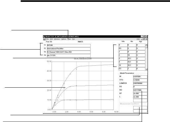
The MODEL window houses all of the functions necessary to create and access data files and to produce optimal models. Its display looks like this:
Pull-down menus
Text fields
Numeric data fields
Model graph
Condition fields
Model fields
Figure 17-1 The Main Display
The principal components of the MODEL window are as follows:
Text fields: There are four Text fields: 'T1', 'T2', 'T3', and 'T4'. The 'T1' and 'T3' fields are imported to MC7 model libraries. The 'T1' field holds the part name and is used in sorting. The other text fields serve only as additional documentation.
Numeric data fields: There are from one to three data fields, depending upon the device type and graph. From one to fifty data sets may be entered in the fields. The data is usually obtained from a data sheet graph. If the graph is not available, a single data point may be taken from the specification tables. If the specification value is not available, no data is entered and default values are used for the corresponding model parameters.
Model Graph: The model graph shows a plot of the curve for the model parameters in the Model fields. It also plots the numeric data points, if any are entered by the user. The quality of the fit can be judged by noting how close the data
240 Chapter 17: The MODEL Program
points match the model curve. A more rigorous estimate is shown in the error display just above the text fields. This error figure is the average percentage error of all data points.
Model fields: Model parameters are changed by initialization or optimization, but may also be directly edited. This is sometimes useful to gauge the effect of a model parameter change. Occasionally, it is useful to manually initialize the model parameter values to obtain a better fit than can be obtained by using initialization.
Condition fields: These fields hold the value of any external test condition used in the measurement from which the data points were obtained.
241

The File menu
MODEL uses data files with the extension "MDL". This menu provides functions for managing the data files, SPICE text model files, and MC7 device model files.
•New: (CTRL + N) This creates a new data file containing a single device.
•Open: (CTRL + O) This loads an existing data file from disk.
•Save: (CTRL + S) This saves the current data file to disk.
•Save As: This lets you save the current data file to disk under a new name.
•Paths...: This lets you specify the default path(s) where the program loads and saves its files.
•Create SPICE File: This saves the parameter values as model statements in a text file, using a file name extension of "LIB". They can be accessed in this form by the MC7 simulator, but not by the MC7 Model Editor.
•Create Model Library: This saves the parameter values as a binary data file, using a file name extension of "LBR". They may be accessed in this form by both the MC7 simulator and by the MC7 Model Editor. This form is the preferred form for use by MC7, since it provides faster access to the part model values when MC7 is searching the libraries in preparation for a run.
•Revert: This restores the currently displayed file to the version stored on disk. If you have made many edits to the current file, and want to abandon them and start with a fresh copy of the file, this is the command to use.
•Close (CTRL+ F4): This command closes the current data file.
•Merge: This merges the current data file with one from the disk. The results are displayed in the current data file, but are only saved to disk if requested by the user with a Save or Save As command or when the file is unloaded.
•Sort: This option sorts the current data file using the T1 field.
•File Name: Recently opened files are listed here.
•Exit: (ALT+ F4) This command exits the MODEL program.
242 Chapter 17: The MODEL Program

The Edit menu
This menu provides the commands for editing the data file:
•Undo: (CTRL + Z) Any change to a text field may be reversed with the Undo command. Undo will only reverse the last change.
•Cut: (CTRL + X) This command deletes the selected text and copies it to the clipboard.
•Copy: (CTRL + C) This command copies selected text to the clipboard.
•Paste: (CTRL + V) This command copies the contents of the clipboard starting at the current cursor position.
•Clear: (DELETE) This command deletes the selected items without copying them to the clipboard.
•Select All: (CTRL + A) This command selects all text in the field where the text cursor is.
•Copy Front Window to Clipboard: This copies all or part of the visible portion of the front window in bitmap graphics format to the clipboard.
•Change Polarity: This command lets you change the polarity of the displayed device. For example, you can change the polarity of a bipolar transistor from NPN to PNP, or MOSFET from PMOS to NMOS.
•Add Part: This option lets you add a new part to the current file. The part type is selected from a submenu and added to the end of the file.
•Delete Data: (CTRL + D) This option lets you delete the data pair or data triplet in the data field where the cursor is presently located. It only affects the Numeric Data fields, not the text fields. It is enabled only when the text cursor is located in one of the Numeric Data fields. Note that there is no Copy Part or Delete Part command on this menu. These functions are part of the Parts List dialog box. You can delete one or more parts by selecting them, then cutting or clearing them. You can copy one or more parts by selecting them, copying them to the clipboard, then pasting them into the file.
243

The Windows menu
This menu provides commands for arranging the open files:
•Cascade: (SHIFT + F5) This command cascades open files in an overlapping manner.
•Tile Vertical: (SHIFT + F4) This command vertically tiles the open files in a non-overlapping manner.
•Tile Horizontal: This command horizontally tiles the open files in a
non-overlapping manner.
•Arrange Icons: This command neatly arranges any minimized file icons.
•File names: This lists the open files by name. Choosing one of the files makes it the active or front window.
244 Chapter 17: The MODEL Program

The Options menu
This menu provides the following choices:
•Help Bar: This toggles the display of the Help Bar, a one line window which provides short descriptions of the item at the current mouse location.
•Preferences: These are simple operational preferences.
•File Warning: This provides a warning when closing edited files.
•Sound: This controls the use of sound for warnings.
•Quit Warning: This provides a warning when quitting.
•Time Stamp: This adds a time stamp at the top of the SPICE model statement output file.
•Date Stamp: This adds a date stamp at the top of the SPICE model statement output file.
•Global Settings: The optimizer must achieve these limits before stopping.
•Maximum Relative Per-iteration Error: If the relative difference in the RMS error function from one iteration to the next drops below this value, the optimization will stop. This value is typically 1u to 1m.
•Maximum Percentage Per-iteration Error: If the percentage difference in the RMS error function from one iteration to the next drops below this value, optimization will stop. This value is typically 1u to 1m.
•Maximum Percentage Error: If the actual percentage error of the RMS error function drops below this value, optimization will stop. This value is typically 0.1 to 5.0.
•Model Defaults
This accesses an editor which lets you change the minimum, initial, and maximum values for all model parameters. The minimum and maximum serve as limits on the value of optimized parameters during the optimization process. The initial value is used for initialization prior to optimization.
245
• Color Preferences
This lets you select the color of the curve, data point icons, graph grid, graph background, and numeric scale.
• Auto Scale (F6)
This command automatically scales the plot.
• Manual Scale (F9)
This option lets you manually change the plot scale.
• Step Model Parameters
This option lets you step any of the model parameters to see their effect on the curve. It is a tool for exploring the effect of different model parameters.
246 Chapter 17: The MODEL Program