

Micro-Cap v7.1.6 / RM
.PDFThe View menu
This menu lets you access the different graphs for each part and the parts themselves. The data file can be viewed as a two-dimensional structure. The graphs are arranged from left to right. The parts are arranged from top to bottom. The CTRL + ARROW keys provide a kind of two-dimensional access to the file:
Previous Graph: |
CTRL + LEFT ARROW shows the graph to the left. |
Next Graph: |
CTRL + RIGHT ARROW shows the graph to the right. |
Previous Part: |
CTRL + UP ARROW shows the part above. |
Next Part: |
CTRL + DOWN ARROW shows the part below. |
The graphs and parts are accessed with these options:
• Parts List (CTRL + L ): This command displays a list box showing all of the parts in the current file. Double-clicking on one of the part names displays the part and its data. The menu lets you cut, copy, paste, and delete parts.
To select a part, click on it. To select more than one part, drag the mouse over the part names, or use CTRL + mouse click to toggle the selection state of single parts, or SHIFT + mouse click to toggle the selection state of many parts.
To delete one or more parts, first select them, then cut (CTRL + X) or clear (Del) them.
To copy one or more parts, first select them, then copy them to the clipboard (CTRL + C), then paste (CTRL + V) them to the end of the file.
•Find Part (CTRL + F ): This searches the current file for a part name in the T1 field.
•Previous Part (CTRL + UP ARROW): This shows the prior part.
•Next Part (CTRL + DOWN ARROW): This shows the next part.
•First Part (CTRL + HOME): This shows the first part in the data file.
•Last Part (CTRL + END): This shows the last part in the data file.
•Previous graph (CTRL + LEFT ARROW): This shows the prior graph.
247
•Next Graph (CTRL + RIGHT ARROW): This shows the next graph.
•First Graph (CTRL + SHIFT + LEFT ARROW): This shows the first graph of the current part.
•Last Graph (CTRL + SHIFT + RIGHT ARROW): This shows the last graph of the current part.
•All Graphs: This mode shows all graphs for the part. When you select this option, all graphs are displayed. A list of the graphs is presented at the end of the menu, together with a check mark. You can selectively add or delete graphs by clicking on the graph name. When more than one graph is shown, the data fields shown are for the selected graph. The selected graph is the one whose title is underlined. You can change the selected graph by clicking on the title bar. When you do, the screen shows the appropriate data fields for the graph.
•One Graph at a Time: This mode shows only one graph at a time.
•Graph Names: This portion lists each of the graphs for the part. If the All Graphs option is enabled, clicking on one of the graph names toggles its display status. If the One Graph at a Time option is enabled, clicking on one of the graph names selects it for display.
248 Chapter 17: The MODEL Program

The Run menu
This menu provides control over the initialization and optimization functions:
• Initialize: (CTRL+I) This initializes the model parameter values
for the displayed graph of the part. This is usually the prelude to optimizing.
•Optimize: (CTRL+T) This optimizes the model parameter values to fit the supplied data points. Optimizing is done for the selected graph of the current part. Optimization is done by minimizing the RMS difference between the data points and the plot values predicted by a particular set of parameters.
•Initialize and Optimize All: This first initializes and then optimizes
each part in the data file. If the parts have never been optimized, this is a convenient way of optimizing all parts in the data file.
• Optimize All: This optimizes each part in the file without initialization. If the parts have been optimized one or more times, and you wish to tighten the optimization tolerances to produce a better fit, or possibly you have changed a few data values in the file, but can't remember which have been changed, this option provides a convenient way to re-optimize the entire data file.
249
A bipolar transistor example
To illustrate the use of MODEL, we'll use the 2N3903 transistor. The example is based upon the product data sheet which begins on page 2-3 in the data book,
Motorola Small-Signal Transistors, FETs, and Diodes Device Data Rev 5.
Begin by creating a new file. Select New from the File menu. Use the name "NEW1.MDL". Click on the NPN type option. Click OK. The program creates a new file with one part of the selected type. The cursor is initially in the T1 text field. Type "2N3903". Enter any text you wish in the remaining three text fields.
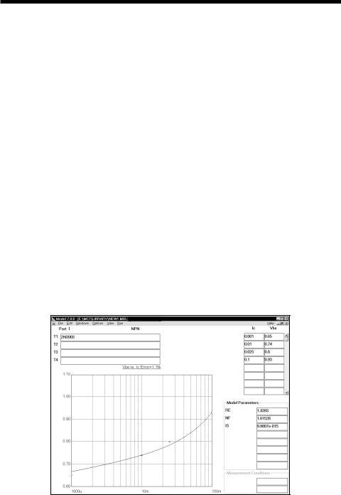
Now you're ready to enter data. Locate Figure 17, the "ON" VOLTAGES graph, on page 2-7 of the Motorola handbook. From the two Vbe vs. Ic plots choose the Vbe(sat) @ Ic/Ib = 10 curve. Press the Tab key or use the mouse to move the cursor to the Ic data field. Enter these data sets from the graph.
Ic |
Vbe |
.001 |
.65 |
.01 |
.74 |
.025 |
.80 |
.1 |
.93 |
Press CTRL + I to initialize and CTRL + T to optimize the values. The results looklikethis:
Figure 17-2 The Vbe vs. Ic plot
250 Chapter 17: The MODEL Program
The model parameters RE, NF, and IS are optimized to produce a fit to the Vbe vs. Ic curve of about 1%. This is a slightly better than average error for this type of graph.
Press CTRL + RIGHT ARROW. This displays the Hoe vs. Ic graph. Use the maximum value of 40 umhos from the table for Hoe.
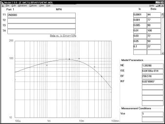
Press CTRL + RIGHT ARROW. This displays the Beta vs. Ic graph. Locate the graph, Figure 15, DC Current Gain, on page 2-6. Select the 25° plot. Enter the following data points from the graph:
Ic |
Beta |
Ic |
Beta |
.0001 |
44 |
.030 |
72 |
.001 |
77 |
.050 |
50 |
.005 |
98 |
.100 |
27 |
.010 |
100 |
|
|
Move the cursor to the Measurement Conditions field and enter 1.0 for Vce. Press CTRL + I to initialize and CTRL + T to optimize. The results look like this:
Figure 17-3 The Beta vs. Ic Plot
The model parameters NE, ISE, BF, and IKF are optimized to fit the plot to within an error of about 11%. A typical error range for this plot is 1% to 20%. Press CTRL + RIGHT ARROW and MODEL will display the next graph, Vce vs. Ic.
251
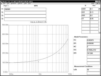
From the same "ON" VOLTAGES graph used earlier, select the Vce(Sat) curve. From the curve enter the following data points:
Ic |
Vce |
.001 |
.1 |
.010 |
.11 |
.05 |
.2 |
.10 |
.35 |
Move the cursor to the Measurement Conditions field and enter 10 for Ic/Ib. Initialize and optimize the values. The results look like this:
Figure 17-4 The Vce vs. Ic Plot
The model parameters RC, BR, NC, ISC, and IKR are optimized to produce a fit to the Vce vs. Ic plot of about 7%. This is a good fit for the Vce plot. Generally an error range of 5% to 25% is to be expected here.
Press CTRL + RIGHT ARROW to select the next plot, Cob vs. Vcb. From Cobo plot in Figure 3, CAPACITANCE graph, on page 2-4 enter these values.
Vcb Cob
0.103.5pf
1.002.7pf
10.01.7pf
Initialize and optimize and the results look like Figure 17-5.
252 Chapter 17: The MODEL Program
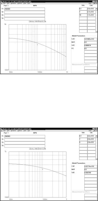
Figure 17-5 The Cob vs. Vcb Plot
Press CTRL + RIGHT ARROW to select the next plot Cib vs. Veb. From Cibo plot in Figure 3, CAPACITANCE graph, on page 2-4, enter these values.
Veb |
Cib |
Veb |
Cib |
Veb |
Cib |
.10 |
4.2pf |
1.0 |
3.3pf |
5.0 |
2.5pf |
Initialize and optimize and the results look like this:
Figure 17-6 The Cib vs. Veb Plot
253
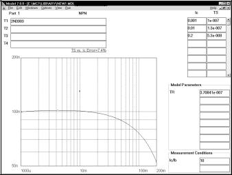
Press CTRL + RIGHT ARROW to select the next plot, TS vs. Ic. From the Ic/Ib = 10 curve in Figure 7, STORAGE TIME, graph on page 2-5, enter these values for collector current and storage time:
Ic |
TS |
1m |
100n |
10m |
130n |
200m |
53n |
Set the Measurement Condition field to 10. Initialize and optimize and the results look like this:
Figure 17-7 The TS vs. Ic Plot
The model parameter TR is optimized to produce an average error of under 10%.
Press CTRL + RIGHT ARROW to select the next plot, FT vs. Ic. From the Small-signal specification tables enter this data point.
Ic |
FT |
10m |
250E6 |
254 Chapter 17: The MODEL Program
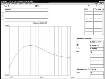
Enter 10.0 for Vce in the Measurement Conditions field. Initialize and optimize and the results look like this:
Figure 17-8 The FT vs. Ic Plot
The model parameters TF and ITF are optimized to produce a near perfect fit to the single data point. Standard, unoptimized XTF and VTF values are used.
This completes the example for the 2N3903. Probably because it is such a popular device, it has a fairly good selection of graphs and specification values to use. Other parts may not be well documented. In these cases, you have three choices:
1.Measure the data sheet values on a sample of actual parts.
2.Use the default model parameter values.
3.Use a part from a different manufacturer with better documentation.
Save the results in a model file using the Save option from the File menu.
The final step is to create a model library file that MC7 can use. Select the Create Model Library option from the File menu. The program will present a Save As dialog box and let you specify the path and name of the model library file to use. Click on the OK button to accept the default name NEW1.LBR. The library file is now saved and ready for use by MC7. Finally, be sure to enter the line
.LIB "NEW1.LBR" into the NOM.LIB text file to tell MC7 about the new file.
Parameters for other device types are created in a similar fashion. A summary of each graph and some guidelines are included in the following pages.
255

Diode graphs
Title |
Forward current vs. Forward voltage |
Purpose |
This screen estimates IS, N, and RS. |
Input |
One or more pairs of If and Vf values. |
Output |
Model values for IS, N, and RS. |
Equations |
Vf = VT•log(If/IS)+If•RS |
Guidelines |
Use data from the If vs. Vf graphs. If unavailable, use typical values |
|
from the tables. Use data from both the low and high current ranges. |
|
The low-current data will determine the value of IS and NF, and the |
|
high-current data points will determine RS. |
Title |
Capacitance C vs. Reverse voltage |
Purpose |
This screen estimates CJO, M, VJ, and FC. |
Input |
One or more pairs of Cj and Vr values. |
Output |
Model values for CJO, M, VJ, and FC. |
Equations |
C = CJO/(1+VR/VJ)M |
Guidelines |
Use data from the C vs. Vr graphs. Vr is the value of the reverse |
|
voltage and is always positive. |
Title |
Id vs Vrev |
Purpose |
This screen estimates RL. |
Input |
One or more pairs of Irev and Vrev values. |
Output |
Model value for RL. |
Equations |
Irev = Vrev/RL (the breakdown portion is ignored) |
Guidelines |
Use data from the Irev vs. Vrev graphs. If unavailable, use typical |
|
values from the tables. RL models the main reverse leakage current |
|
component. BV is not optimized. |
Title |
Trr vs. Ir/If ratio |
Purpose |
This screen estimates TT, the transit time parameter. |
Input |
One or more pairs of Trr and Ir/If values. Ir/If is the ratio of the |
|
forward and reverse base currents used to measure Trr. |
Output |
Model value for TT. |
Equations |
trr = tt•log10(1.0+1.0/ratio) |
Guidelines |
Use data from the Trr vs. Ir/If ratio graphs. If unavailable, use |
|
typical values from the tables. If the typical value is not |
|
available, use an average of the min and max values. |
256 Chapter 17: The MODEL Program