

Micro-Cap v7.1.6 / RM
.PDFaccomplished by increasing the Number of Points value or decreasing the frequency range and centering it near the expected notch frequency.
Plotting reactive power:
To plot reactive power through a capacitor C1, plot V(C1)*I(C1). To plot reactive power through an inductor L1, plot V(L1)*I(L1). For a port whose input nodes are A and B, plot (V(A,B))*I(V1), where V1 is a zero-volt independent voltage source in series with one of the port leads.
Using the P key
During an AC analysis run, the value of the expressions for each curve can be seen by pressing the 'P' key. This key toggles the printing of the numeric values on the analysis plot adjacent to the expressions. This is a convenient way to check the course of a new, lengthy simulation when the initial plot scales are unknown. This feature may significantly slow the simulation, so only use it to "peek" at the numeric results, then toggle it off with the 'P' key.
137
138 Chapter 7: AC Analysis

Chapter 8 |
DC Analysis |
What's in this chapter
This chapter describes the features of DC analysis. DC is an acronym for direct current, one of two competing power transmission strategies early in the development of electrical engineering technology. For our purposes, DC means simply that the sources are constant and do not vary with time.
During a DC analysis, capacitors are open-circuited, inductors are short-circuited, and sources are set to their time-zero values. DC analysis sweeps one or two input independent variables (such as current or voltage source values) over a specified range. At each voltage or current step, MC7 performs an operating pointcalculation.
Transfer characteristics are a typical application for DC analysis.
Features new in Micro-Cap 7
•Optimizer
•Watch window
•Breakpoints window
•Range format <high> [,<low>] [,<grid spacing>] [,<bold spacing>].
139
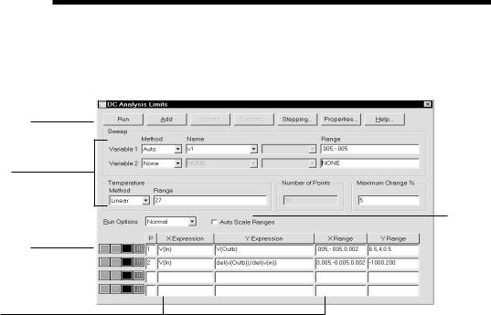
The DC Analysis Limits dialog box
The Analysis Limits dialog box is divided into five major areas: the Command buttons, Numeric limits, Curve options, Expression fields, and Options.
Command buttons
Numeric limits
Options
Curve options
Expressions
Figure 8-1 The Analysis Limits dialog box
Command buttons provide these commands.
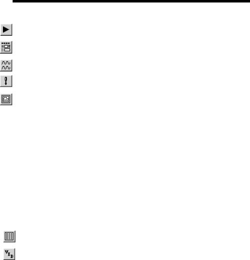
Run: This command starts the analysis run. Clicking the Tool bar Run  button or pressing F2 will also start the run.
Add: This command adds another Curve options field and Expressions field line after the line containing the cursor. The scroll bar to the right of the Expressions field scrolls through the curves when needed.
Delete: This command deletes the Curve option field and Expressions field line where the text cursor is.
Expand: This command expands the working area for the text field where the text cursor currently is. A dialog box is provided for editing or viewing. To use the feature, click in an expression field, then click the Expand button.
Stepping: This command calls up the Stepping dialog box. Stepping is reviewed in a separate chapter.
140 Chapter 8: DC Analysis
Properties: This command invokes the Properties dialog box which lets you control the analysis plot window and the way curves are displayed.
Help: This command calls up the Help system.
The definition of each field in the Numeric limits are as follows:
• Variable 1: This row specifies the Method, Name, and Range fields for variable 1. Its value is usually plotted along the X axis. Each value produces a minimum of one data point per curve. There are four column fields for this variable.
• Method: This field specifies one of four methods for stepping the variable: Auto, Linear, Log, or List.
•Auto: In Auto mode the rate of step size is adjusted to keep the point-to-point change less than Maximum Change % value.
•Linear: This mode uses the following syntax from the Range column for this row:
<end> [,<start> [,<step>] ]
Start defaults to 0.0. Step defaults to (start - end)/50. Variable 1 starts at start. Subsequent values are computed by adding step until end is reached.
• Log: Log mode uses the following syntax from the Range column for this row:
<end> [,<start> [,<step>] ]
Start defaults to end/10. Step defaults to exp(ln(end/start)/10). Variable 1 starts at start. Subsequent values are computed by multiplying by step until end is reached.
• List: List mode uses the following syntax from the Range column for this row:
<v1> [,<v2> [,<v3>] ...[,<vn>] ]
The variable is simply set to each of the values v1, v2, .. vn.
141
•Name: This field specifies the name of variable 1. The variable itself may be a source value, temperature, a model parameter, or a symbolic parameter (one created with a .DEFINE statement). Model parameter stepping requires both a model name and a model parameter name.
•Range: This field specifies the numeric range for the variable. The range syntax depends upon the Method field described above.
•Variable 2: This row specifies the Method, Name, and Range fields for variable 2. The syntax is the same as for variable 1, except that the stepping options include None and exclude Auto. Step defaults to (start - end)/10. Each value of variable 2 produces a separte branch of the curve.
•Temperature: This controls the temperature of the run. The fields are:
•Method: This field specifies one of two methods for stepping the temperature: Linear or List.
• Linear: This mode uses the following syntax from the Range column for this row:
<end> [,<start> [,<step>] ]
Start defaults to end. Step defaults to start - end. Temperature begins at start. Subsequent values are computed by adding step untilend is reached.
• List: List mode uses the following syntax from the Range column for this row:
<v1> [,<v2> [,<v3>] ...[,<vn>] ]
Temperature is simply set to each of the values v1, v2, .. vn.
One run is produced for each temperature. Note that when temperature is selected as one of the stepped variables (variable1 or variable 2) this field is not available.
• Range: This field specifies the range for the temperature variable. The range syntax depends upon the Method field described above.
142 Chapter 8: DC Analysis
• Number of Points: This is the number of data points to be interpolated and printed if numeric output is requested. This number defaults to 51 and is often set to an odd value to produce an even print interval. Its value is:
(<final1> - <initial1> ) /(<Number of points> - 1)
<Number of points> values are printed for each value of the Variable 2 source.
• Maximum Change %: This value is only used if Auto is selected as the step method for Variable 1.
The Curve options are located below the Numeric limits and to the left of the Expressions. Curve options affect the curve in the same row. The definition of each option is as follows:
The first option toggles the X-axis between a linear  and a log
  plot. Log plots require positive scale ranges.
The second option toggles the Y-axis between a linear  and a log
  plot. Log plots require positive scale ranges.
The  option activates the color menu. There are 64 color choices for an individual curve. The button color is the curve color.
The  option prints a table showing the numeric value of the curve. The number of values printed is set by the Number of Points value. The table is printed to the Output window and saved in the file CIRCUITNAME.DNO.
A number from 1 to 9 in the Plot (P) column places the curve into a plot group. All curves with like numbers are placed in the same plot group. If the P column is blank, the curve is not plotted.
The Expressions field is used to specify the horizontal (X) and vertical (Y) scale ranges and expressions. Some common expressions used are VCE(Q1) (collector to emitter voltage of transistor Q1) or IB(Q1) (base current of transistor Q1).
The X Range and Y Range fields specify the scales to be used when plotting the X and Y expressions.
143
The range format is:
<high> [,<low>] [,<grid spacing>] [,<bold grid spacing>]
<low> defaults to zero. [,<grid spacing>] sets the spacing between grids. [,<bold grid spacing>] sets the spacing between bold grids. Placing "AUTO" in the scale range calculates that individual range automatically. The Auto Scale Ranges option calculates scales for all ranges during the simulation run and updates the X and Y Range fields. The Auto Scale (F6) command immediately scales all curves, without changing the range values, letting you restore them with CTRL + HOME if desired. Note that <grid spacing> and <bold grid spacing> are used only on linear scales. Logarithmic scales use a natural grid spacing of 1/ 10 the major grid values and bold is not used. The Auto Scale command uses the
Preferences / Auto Scale Grids value to set the grid spacing.
Clicking the right mouse button in the Y expression field invokes the Variables list which lets you select variables, constants, functions, and operators, or expand the field to allow editing long expressions. Clicking the right mouse button in the other fields invokes a simpler menu showing suitable choices.
The Options area is below the Numeric limits. The Auto Scale Ranges option has a check box. Clicking the mouse in the box will toggle the options on or off with an X in the box showing that the option is enabled.
The options available from here are:
•Run Options
•Normal: This runs the simulation without saving it to disk.
•Save: This runs the simulation and saves it to disk.
•Retrieve: This loads a previously saved simulation and plots and prints it as if it were a new run.
•Auto Scale Ranges: This sets the X and Y range to auto every time a simulation is run. If it is disabled, the values from the range fields will be used.
144 Chapter 8: DC Analysis
The DC menu
Run: (F2) This starts the analysis run.
Limits: (F9) This accesses the Analysis Limits dialog box.
Stepping: (F11) This accesses the Stepping dialog box.
Optimize: (CTRL + F11) This accesses the Optimize dialog box.
Analysis Window: (F4) This command displays the analysis plot.
Watch: (CTRL + W) This displays the Watch window where you define expressions or variables to watch during a breakpoint invocation.
Breakpoints: (ALT + F9) This accesses the Breakpoints dialog box. Breakpoints are Boolean expressions that define when the program will enter single-step mode so that you can watch specific variables or expressions. Typical breakpoints are V(A)>=1 AND V(A)<=1.5, and V(OUT)>5.5.
3D Windows: This lets you add or delete a 3D plot window. It is enabled only if more than one run is done.
Performance Windows: This lets you add or delete a performance plot window. It is enabled only if there is more than one run.
Numeric Output: (F5) This shows the Numeric Output window.
State Variables editor: (F12) This accesses the State Variables editor.
Reduce Data Points: This item invokes the Data Point Reduction dialog box. It lets you delete every n'th data point. This is useful when you use very small time steps to obtain very high accuracy, but do not need all of the data points produced. Once deleted, the data points cannot be recovered.
Exit Analysis: (F3) This exits the analysis.
145
Numeric output
Numeric output may be obtained for the X and Y expressions of each curve by clicking the Numeric Output button  in the curve row. Numeric output includes:
Analysis Limits Summary: This is a printout of the main analysis limits from the Analysis Limits, Stepping, and Monte Carlo dialog boxes.
Expression tables: This is a tabular printout of the value of each X and Y expression of each selected curve. Duplicated X expressions are eliminated. The values are interpolated from the actual data points. The Number of Points value from the Analysis Limits dialog box determines the number of points printed in the table.
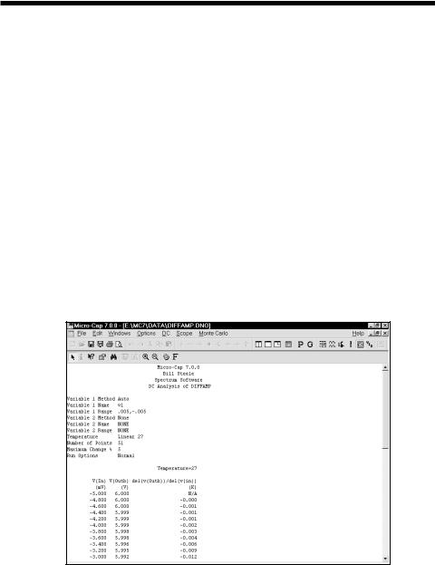
Output is saved to the text file CIRCUITNAME.DNO and printed to the Numeric Output window. This window is accessible after the run from the DC menu. Here is a typical numeric output window.
Figure 8-2 Numeric output
146 Chapter 8: DC Analysis