7.2 Origin and Consequences of Magnetic Order |
387 |
|
|
Consider a magnetized material in which there is no real or displacement current. The two relevant Maxwell equations can be written in the absence of external currents and in the static situation
H = 0 , |
(7.127) |
B = 0 . |
(7.128) |
Equation (7.127) implies there is a potential Φ from which the magnetic field H can be derived:
We assume a constitutive equation linking the magnetic induction B, the magnetization M and H;
B = μ0 (H + M ) , |
(7.130) |
where μ0 is called the permeability of free space. Equations (7.128) and (7.130) become
H = − M . |
(7.131) |
In terms of the magnetic potential Φ, |
|
2Φ = M . |
(7.132) |
This is analogous to Poisson’s equation of electrostatics with ρM = − ·M playing the role of a magnetic source density.
By analogy to electrostatics, and in terms of equivalent surface and volume pole densities, we have
Φ = |
1 |
∫ |
M dS − ∫ |
M dV |
|
, |
(7.133) |
|
|
|
|
|
S |
r |
V |
r |
|
|
|
4π |
|
|
|
|
|
where S and V refer to the surface and volume of the magnetized body. By analogy to electrostatics the magnetostatic self-energy is
|
UM = |
μ0 |
∫ ρMΦdV = − |
μ0 |
∫ MΦdV = − |
μ0 |
∫ M ΗdV |
|
|
2 |
2 |
2 |
(7.134) |
|
|
|
|
|
|
|
|
|
|
(since ∫ |
(MΦ)dV = 0), |
|
|
|
|
|
|
all space |
|
|
|
|
which also would follow directly from the energy of a dipole μ in a magnetic field (−μ·B), with a 1/2 inserted to eliminate double counting. Using ·M = − ·H and ∫all space ·(HΦ)dV = 0, we get
|
UM = |
μ0 |
∫ H 2dV . |
(7.135) |
|
2 |
|
|
|
|
388 7 Magnetism, Magnons, and Magnetic Resonance
For ellipsoidal specimens the magnetization is uniform and |
|
H D = −DM , |
(7.136) |
where HD is the demagnetization field, D is the demagnetization factor that depends on the shape of the sample and the direction of magnetization and hence one has shape isotropy, since (7.135) would have different values for M in different directions. For ellipsoidal magnets, the demagnetization energy per unit volume is then
uM = |
μ0 |
D |
2 |
M |
2 |
. |
(7.137) |
2 |
|
|
|
|
|
|
|
|
|
7.2.3 Spin Waves and Magnons (B)
If there is an external magnetic field B = μ0Hzˆ, and if the magnetic moment of each atom is m = 2μS (2μ ≡ −gμB 14 in previous notation), then the above consid-
erations tell us that the Hamiltonian describing an (nn) exchange coupled spin system is
H = −J ∑ j S j S j + − 2μ0μH ∑ j S jz . |
(7.138) |
j runs over all atoms, and δ runs over the nearest neighbors of j, and also we may redefine J so as to write (7.138) as H = (J/2)∑…. (We do this sometimes to emphasize that (7.138) double counts each interaction.) From now on it will be assumed that there exist real solids for which (7.138) is applicable. The first term in this equation is the Heisenberg Hamiltonian and the second term is the Zeeman energy.
Let
S 2 = (∑ j S j )2 , |
(7.139) |
and |
|
Sz = ∑ j S jz . |
(7.140) |
Then it is possible to show that the total spin and the total z component of spin are constants of the motion. In other words,
[H , S 2 ] = 0 , |
(7.141) |
and |
|
[H , Sz ] = 0 . |
(7.142) |
14 The minus sign comes from the negative charge on the electron.
7.2 Origin and Consequences of Magnetic Order |
389 |
|
|
Spin Waves in a Classical Heisenberg Ferromagnet (B)
We want to calculate the internal energy u (per spin) and the magnetization M. Assuming the magnetization is in the z direction and letting A stand for the quan- tum-statistical average of A, we have (if H = 0)
u = 1 |
H = − 1 ∑i, j Jij |
Si S j , |
(7.143) |
N |
2N |
|
|
and |
|
|
|
|
M = − gμB ∑iz Siz |
, |
(7.144) |
|
V |
|
|
(with the S written in units of |
and V is the volume of the crystal and Jij absorbs |
an 2) where the Heisenberg Hamiltonian is written in the form |
|
H = − 12 ∑i, j Jij Si S j .
Using the fact that
S 2 = Sx2 + S y2 + Sz2 ,
assuming a ferromagnetic ground state, and very low temperatures (where spin wave theory is valid) so that Sx and Sy are very small,
Sz = − S 2 − Sx2 − S y2 ,
(negative so M > 0) and thus
|
|
|
|
2 |
2 |
|
|
|
Sz −S |
|
1 |
− |
Sx |
+ S y |
|
, |
(7.145) |
|
2S 2 |
|
|
|
|
|
|
|
|
|
|
which can be substituted in (7.144). Then by (7.143)
u − |
1 |
∑ |
|
S 2 J |
|
|
i, j |
ij |
1 |
|
2N |
|
|
|
|
|
|
|
|
|
|
− |
1 ∑i, j Jij Six S jx + Siy S jy . |
|
|
2N |
|
|
|
|
We obtain |
|
|
|
|
|
|
M = |
N gμBS − gμB ∑i |
Six2 + Siy2 , |
(7.146) |
|
|
V |
2SV |
|
|
u = − S 2 Jz + |
1 |
∑i, j Jij Six2 + Siy2 |
− SixS jx − Siy S jy , |
(7.147) |
|
2 |
2N |
|
|
|
390 7 Magnetism, Magnons, and Magnetic Resonance
where z is the number of nearest neighbors. It is now convenient to Fourier transform the spins and the exchange integral
Si = ∑k Skeik R
J (k) = ∑R J (R)eiq R .
Using the standard crystal lattice mathematics and S−kx = S*kx, we find:
M |
= |
N |
|
|
|
− |
1 |
|
|
|
V |
gμBS 1 |
2S |
∑k SkxSkx + Sky Sky |
|
|
|
|
|
|
|
|
|
|
u = − |
S 2 Jz |
+ |
1 |
∑k (J (0) − J (k)) SkxSkx |
+ SkySky . |
|
2 |
|
|
2 |
|
|
|
|
|
|
|
(7.148)
(7.149)
(7.150)
(7.151)
We still have to evaluate the thermal averages. To do this, it is convenient to exploit the analogy of the spin waves to a set of uncoupled harmonic oscillators whose energy is proportional to the amplitude squared. We do this by deriving the equations of motion and showing in our low-temperature “spin-wave” approximation that they are harmonic oscillators. We can write the Heisenberg Hamiltonian equation as
|
|
1 |
|
Si |
|
|
H |
= − |
2 |
∑ j ∑i Jij |
|
(−gμB S j ) , |
(7.152) |
|
|
|
|
− gμB |
|
where −gμBSj is the magnetic moment. The 1/2 takes into account the double counting and we therefore identify the effective field acting on Sj as
BM |
|
= − |
1 |
∑i Jij Si . |
(7.153) |
j |
|
|
|
gμB |
|
Treating the Si as dimensionless so Si is the angular momentum, and using the fact that torque is the rate of change of angular momentum and is the moment crossed into field, we have for the equations of motion
|
dS j |
= ∑i Jij S j × Si . |
(7.154) |
|
dt |
|
|
|
We leave as a problem to show that after Fourier transformation the equations of motion can be written:
|
dSk |
= ∑k′′ J (k′′)Sk −k′′ × Sk′′ . |
(7.155) |
|
dt |
|
|
|
For the ferromagnetic ground state at low temperature, we assume that
Sk =0 >> Sk ≠0 ,
7.2 Origin and Consequences of Magnetic Order |
391 |
|
|
since
Sk =0 = N1 ∑R SR ,
and at absolute zero,
ˆ |
= 0 . |
Sk =0 = Sk , Sk ≠0 |
Even with small excitations, we assume S0z = S, S0x = S0y = 0 and Skx, Sky are of first order. Retaining only quantities of first order, we have
|
dSkx |
= S[J (0) − J (k)] Sky |
(7.156a) |
|
dt |
|
|
|
|
|
dSky |
|
= −S[J (0) − J (k)] Skx |
(7.156b) |
|
dt |
|
|
|
|
|
|
|
|
|
dSkz |
= 0 . |
(7.156c) |
|
|
|
|
|
|
|
|
|
dt |
|
Combining (7.156a) and (7.156b), we obtain harmonic-oscillator-type equations with frequencies ω(k) and energies ε(k) given by
ε(k) = ω(k) = S[J (0) − J (k)] . |
(7.157) |
Combining this result with (7.151), we have for the average energy per oscillator,
u = − S 2 Jz |
+ |
1 |
∑k |
ε(k) |
| Skx |2 + | Sky |2 |
2 |
|
2 |
|
S |
|
for z nearest neighbors. For quantized harmonic oscillators, up to an additive term, the average energy per oscillator would be
|
|
1 |
∑k ε(k) nk . |
|
|
|
|
N |
|
|
|
|
|
|
|
|
Thus, we identify nk as |
|
|
|
|
|
|
|
|
|
|
|
| Skx |2 + | Sky |2 |
N , |
|
|
|
|
|
|
2S |
|
|
|
|
|
|
|
|
|
|
|
|
|
|
|
and we write (7.150) and (7.151) as |
|
|
|
|
|
|
|
|
M = |
N |
|
|
|
− |
1 |
∑k nk |
|
(7.158) |
V |
gμBS 1 |
NS |
|
|
|
|
|
|
|
|
|
|
u = − S 2 Jz |
+ 1 |
|
∑k ε |
(k) nk |
. |
(7.159) |
|
|
2 |
|
N |
|
|
|
|
|
392 7 Magnetism, Magnons, and Magnetic Resonance
Now nk is the average number of excitations in mode k (magnons) at temperature
T.
By analogy with phonons (which represent quanta of harmonic oscillators) we say
|
nk |
= |
1 |
. |
(7.160) |
|
eε(k) / kT |
|
|
|
−1 |
|
As an example, we work out the consequences of this for simple cubic lattices with Z = 6 and nearest-neighbor coupling.
J (k) = ∑ J (R)eik R = 2J (cos kxa + cos k ya + cos kza).
At low temperatures where only small k are important, we find
ε(k) = S [J (0) − J (k)] SJk 2a2 . |
(7.161) |
We will evaluate (7.158) and (7.159) using (7.160) and (7.161) later after treating spin waves quantum mechanically from the beginning.
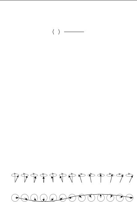
The name “spin-waves” comes from the following picture. In Fig. 7.10, suppose
Skx = S sin(θ) exp[iω(k)t] ,
then
Skx = iω(q) Skx = ω(k) Sky
by the equation of motion. So,
iSkx = Sky .
Therefore, if we had one spin-wave mode q in the x direction, e.g., then
SRx = exp(ik R)Skx = S sin(θ) exp[i(kRx +ωt)], SRy = S sin(θ) exp[i(kRx +ωt −π / 2)].
(a)
 a
a

(b)
Fig. 7.10. Classical representation of a spin wave in one dimension (a) viewed from side and (b) viewed from top (along –z). The phase angle from spin to spin changes by ka. Adapted from Kittel C, Introduction to Solid State Physics, 7th edn, Copyright © 1996 John Wiley and Sons, Inc. This material is used by permission of John Wiley and Sons, Inc
7.2 Origin and Consequences of Magnetic Order |
393 |
|
|
Thus, if we take the real part, we find
SRx = S sin(θ) cos(kRx + ωt),
SRy = S sin(θ)sin(kRx + ωt),
and the spins all spin with the same frequency but with the phase changing by ka, which is the change in kRx, as we move from spin to spin along the x-axis.
As we have seen, spin waves are collective excitations in ordered spin systems. The collective excitations consist in the propagation of a spin deviation, θ. A localized spin at a site is said to undergo a deviation when its direction deviates from the direction of magnetization of the solid below the critical temperature. Classically, we can think of spin waves as vibrations in the magnetic moment density. As mentioned, quanta of the spin waves are called magnons. The concept of spin waves was originally introduced by F. Bloch, who used it to explain the temperature dependence of the magnetization of a ferromagnet at low temperatures. The existence of spin waves has now been definitely proved by experiment. Thus the concept has more validity than its derivation from the Heisenberg Hamiltonian might suggest. We will only discuss spin waves in ferromagnets but it is possible to make similar comments about them in any ordered magnetic structure. The differences between the ferromagnetic case and the antiferromagnetic case, for example, are not entirely trivial [60, p 61].
Spin Waves in a Quantum Heisenberg Ferromagnet (A)
The aim of this section is rather simple. We want to show that the quantum Heisenberg Hamiltonian can be recast, in a suitable approximation, so that its energy excitations are harmonic-oscillator-like, just as we found classically (7.161).
Here we make two transformations and a long-wavelength, low-temperature approximation. One transformation takes the Hamiltonian to a localized excitation description and the other to an unlocalized (magnon) description. However, the algebra can get a little complex.
Equation (7.138) (with = 1 or 2μ = −gμB) is our starting point for the threedimensional case, but it is convenient to transform this equation to another form for calculation. From our previous discussion, we believe that magnons are similar to phonons (insofar as their mathematical description goes), and so we might guess that some sort of second quantization notation would be appropriate. We have already indicated that the squared total spin and the z component of total spin give good quantum numbers. We can also show that Sj2 commutes with the Heisenberg Hamiltonian so that its eigenvalues S(S + 1) are good quantum numbers. This makes sense because it just says that the total spin of each atom remains constant. We assume that the spin S of every ion is the same. Although each atom has three components of each spin vector, only two of the components are independent.
394 7 Magnetism, Magnons, and Magnetic Resonance
The Holstein and Primakoff Transformation (A) Holstein and Primakoff15 have developed a transformation that not only has two independent variables, but also utilizes the very convenient second quantization notation. The Holstein– Primakoff transformation is also very useful for obtaining terms that describe magnon–magnon interactions.16 This transformation is (with = 1 or S representing S/ ):
S +j ≡ S jx +
S −j ≡ S jx −
|
|
|
|
† |
|
|
1/ 2 |
iS jy = |
2S |
|
− |
a j a j |
|
a j |
1 |
2S |
|
|
|
|
|
|
|
|
|
|
|
|
|
|
|
|
a†a |
1/ 2 |
iS jy = |
|
† |
|
|
j |
|
j |
2S a j 1− |
|
2S |
|
|
|
|
|
|
|
|
|
|
S jz ≡ S − a†j a j .
We could use these transformation equations to attempt to determine what properties aj and aj† must have. However, it is much simpler to define the properties of the aj and aj† and show that with these definitions the known properties of the Sj operators are obtained. We will assume that the a† and a are boson creation and annihilation operators (see Appendix G) and hence they satisfy the commutation relations
[a j , al† ] = δ lj . |
(7.165) |
We first show that (7.164) is consistent with (7.162) and (7.163). This amounts to showing that the Holstein–Primakoff transformation automatically puts in the constraint that there are only two independent components of spin for each atom. We start by dropping the subscript j for a particular atom and by using the fact that Sj2 has a good quantum number so we can substitute S(S + 1) for Sj2 (with = 1). We can then write
S(S +1) = Sx2 + S y2 + Sz2 = Sz2 + 12 (S +S − + S −S + ) .
By use of (7.162) and (7.163) we can use (7.166) to calculate Sz2. That is,
Sz2 =
|
|
|
a |
† |
a |
1/ 2 |
|
|
|
|
a |
† |
a |
1/ 2 |
|
|
|
|
a |
† |
a |
|
|
|
|
|
|
|
|
|
|
† |
|
|
|
|
+ a |
† |
|
|
|
|
a |
|
|
S(S +1) − S |
|
1− |
|
|
|
|
(1+ a |
|
a) 1 |
− |
|
|
|
|
|
1 |
− |
|
|
|
|
|
. |
|
|
2S |
|
|
|
|
2S |
|
|
|
2S |
|
|
|
|
|
|
|
|
|
|
|
|
|
|
|
|
|
|
|
|
|
|
|
|
|
|
|
|
|
|
|
|
|
|
|
|
|
|
|
|
|
|
|
|
|
|
|
|
|
|
|
|
|
|
|
|
|
|
|
|
|
|
|
|
|
|
|
|
|
|
15See, for example, [7.38].
16At least for high magnetic fields; see Dyson [7.18].
7.2 Origin and Consequences of Magnetic Order |
395 |
|
|
Remember that we define a function of operators in terms of a power series for the
function, and therefore it is clear that a†a will commute with any function of a†a. Also note that [a†a, a] = a†aa − aa†a = a†aa − (1 + a†a)a = −a, and so we can
transform (7.167) to give after several algebraic steps:
Sz2 = (S − a†a)2 . |
(7.168) |
Equation (7.168) is consistent with (7.164), which was to be shown.
We still need to show that Sj+ and Sj− defined in terms of the annihilation and creation operators act as ladder operators should act. Let us define an eigenket of
Sj2 and Sjz, by (still with |
= 1) |
|
|
|
|
|
|
|
|
|
|
S 2j S,ms = S(S +1) S,ms |
, |
|
|
(7.169) |
and |
|
|
|
|
|
|
|
|
|
|
|
|
|
S jz |
S, ms = ms |
S, ms . |
|
|
|
(7.170) |
Let us further define a spin-deviation eigenvalue by |
|
|
|
|
|
|
|
|
|
n = S − ms , |
|
|
|
(7.171) |
and for convenience let us shorten our notation by defining |
|
|
|
|
|
|
|
|
n = S, ms . |
|
|
|
(7.172) |
By (7.162) we can write |
|
|
|
|
|
|
|
|
+ |
|
|
† |
1/ 2 |
|
n −1 |
1/ 2 |
|
|
|
− |
a j a j |
a j n = |
|
n n −1 , |
(7.173) |
S j n = |
2S 1 |
2S |
|
2S 1− |
2S |
|
|
|
|
|
|
|
|
|
|
|
|
|
|
|
|
|
|
|
|
|
where we have used aj|n = n1/2|n − 1 and also the fact that |
|
|
|
|
|
a†j a j |
n |
= (S − S jz ) n = n n . |
|
|
(7.174) |
By converting back to the |S, ms notation, we see that (7.173) can be written |
|
S +j S, ms |
= |
(S − ms )(S + ms +1) |
S, ms +1 . |
|
(7.175) |
Therefore Sj+ does have the characteristic property of a ladder operator, which is what we wanted to show. We can similarly show that the Sj− has the step-down ladder properties.
Note that since (7.175) is true, we must have that
S + S,ms = S = 0 . |
(7.176) |
396 7 Magnetism, Magnons, and Magnetic Resonance
A similar calculation shows that
S − S,−ms = S = 0 . |
(7.177) |
We needed to assure ourselves that this property still held even though we defined the S+ and S− in terms of the aj† and aj. This is because we normally think of the a as operating on |n , where 0 ≤ n ≤ ∞. In our situation we see that 0 ≤ n < 2S + 1. We have now completed the verification of the consistency of the Holstein– Primakoff transformation. It is time to recast the Heisenberg Hamiltonian in this new notation.
Combining the results of Problem 7.10 and the Holstein–Primakoff transformation, we can write
H =
|
|
|
|
|
|
|
|
|
|
|
|
† |
|
|
1/ 2 |
|
|
† |
|
1/ 2 |
|
|
† |
|
† |
|
|
|
|
|
|
|
|
|
|
a j + |
|
|
|
|
|
|
|
† |
|
|
a j a j |
|
|
|
a j + |
|
|
− J ∑ j (S |
− a j a j )(S − a j + |
a j + |
) + S a j 1 |
− |
|
|
|
|
1 |
− |
|
|
|
a j+δ |
2S |
|
|
2S |
|
|
|
|
|
|
|
|
|
|
|
|
|
|
|
|
|
|
|
|
|
|
|
|
|
|
|
|
|
|
|
|
|
|
|
|
|
|
|
|
|
|
|
|
|
|
|
|
|
|
|
|
|
|
|
|
|
|
|
|
|
|
|
† |
1/ 2 |
|
|
|
† |
|
|
1/ 2 |
|
|
|
|
|
|
|
|
|
|
† |
|
+ |
a j + |
|
|
|
|
|
|
|
|
|
|
|
† |
|
|
a j a j |
|
|
a j |
|
|
|
|
|
|
|
|
|
+ 1 |
− |
|
|
a ja j + |
1 |
− |
|
|
|
|
|
|
|
|
+ gμB |
(μ0H )∑ j (S − a j a j ) . |
2S |
|
2S |
|
|
|
|
|
|
|
|
|
|
|
|
|
|
|
|
|
|
|
|
|
|
|
|
|
|
|
|
|
|
|
|
|
|
|
|
|
|
|
|
|
|
|
|
|
|
|
|
|
|
|
|
|
|
|
|
|
|
|
|
|
|
|
(7.178) Equation (7.178) is the Heisenberg Hamiltonian (plus a term for an external magnetic field) expressed in second quantization notation. It seems as if the problem has been complicated rather than simplified by the Holstein–Primakoff transformation. Actually both (7.138) and (7.178) are equally impossible to solve exactly. Both are many-body problems. The point is that (7.178) is in a form that can be approximated fairly easily. The approximation that will be made is to expand the square roots and concentrate on low-order terms. Before this is done, it is convenient to take full advantage of translational symmetry. This will be done in the next section.
Magnons (A) The aj† create localized spin deviations at a single site (one atom per unit cell is assumed). What we need (in order to take translational symmetry into account) is creation operators that create Bloch-like nonlocalized excitations. A transformation that will do this is
Bk = |
1 |
∑ j exp(ik R j )a j |
, |
(7.179a) |
|
N |
|
|
|
and |
|
|
|
|
Bk† = |
1 |
∑ j exp(−ik R j )a†j |
, |
(7.179b) |
|
N |
|
|
|