Metals are one of our most important sets of materials. The study of bronzes (alloys of copper and tin) dates back thousands of years. Metals are characterized by high electrical and thermal conductivity and by electrical resistivity (the inverse of conductivity) increasing with temperature. Typically, metals at high temperature obey the Wiedeman–Franz law (Sect. 3.2.2). They are ductile and deform plastically instead of fracturing. They are also opaque to light for frequencies below the plasma frequency (or the plasma edge as discussed in the chapter on optical properties). Many of the properties of metals can be understood, at least partly, by considering metals as a collection of positive ions in a sea of electrons (the jellium model). The metallic bond, as discussed in Chap. 1, can also be explained to some extent with this model.
Metals are very important but this chapter is relatively short. The reason for this is that various properties of metals are discussed in other chapters. For example in Chap. 3 the free-electron model, the pseudopotential, and band structure were discussed, as well as some aspects of electron correlations. Electron correlations were also mentioned in Chap. 4 along with the electrical and thermal conductivity of solids including metals. Metals are also important for the study of magnetism (Chap. 7) and superconductors (Chap. 8). The effect of electron screening is discussed in Chap. 9 and free-carrier absorption by electrons in Chap. 10.
Metals occur whenever one has partially filled bands because of electron concentration and/or band overlapping. Many elements and alloys form metals (see Sect. 5.10). The elemental metals include alkali metals (e.g. Na), noble metals (Cu and Ag are examples), polyvalent metals (e.g. Al), transition metals with incomplete d shells, rare earths with incomplete f shells, lanthanides, and actinides. Even nonmetallic materials such as iodine may become metallic under very high pressure.
Also, in this chapter we will include some relatively new and novel ideas such as heavy electron systems, and so-called linear metals.
We start by discussing one of the most important properties of metals—the Fermi surface, and show how one can use simple free-electron ideas along with the Brillouin zone to get a first orientation.
5.1 Fermi Surface (B)
Mackintosh has defined a metal as a solid with a Fermi-Surface [5.19]. This tacitly assumes that the highest occupied band is only partly filled. At absolute zero, the Fermi surface is the highest filled energy surface in k or wave vector space.
266 5 Metals, Alloys, and the Fermi Surface
When one has a constant potential, the metal has free-electron spherical energy surfaces, but a periodic potential can cause many energy surface shapes. Although the electrons populate the energy surfaces according to Fermi–Dirac statistics, the transition from fully populated to unpopulated energy surfaces is relatively sharp at room temperature. The Fermi surface at room temperature is typically as well defined as is the surface of a peach, i.e. the surface has a little “fuzz”, but the overall shape is well defined.
For many electrical properties, only the electrons near the Fermi surface are active. Therefore, the nature of the Fermi surface is very important. Many Fermi surfaces can be explained by starting with a free-electron Fermi surface in the ex- tended-zone scheme and, then, mapping surface segments into the reduced-zone scheme. Such an approach is said to be an empty-lattice approach. We are not considering interactions but we have already noted that the calculations of Luttinger and others (see Sect. 3.1.4) indicate that the concept of a Fermi surface should have meaning, even when electron–electron interactions are included. Experiments, of course, confirm this point of view (the Luttinger theorem states that the volume of the Fermi surface is unchanged by interactions).
When Fermi surfaces intersect Brillouin zone boundaries, useful Fermi surfaces can often be constructed by using an extended or repeated-zone scheme. Then con- stant-energy surfaces can be mapped in such a way that electrons on the surface can travel in a closed loop (i.e. without “Bragg scattering”). See, e.g. [5.36, p. 66].
Going beyond the empty-lattice approach, we can use the results of calculations based on the one-electron theory to construct the Fermi surface. We first solve the Schrödinger equation for the crystal to determine Eb(k) for the electrons (b labels the different bands). We assume the temperature is zero and we find the highest occupied band Eb′(k). For this band, we construct constant-energy surfaces in the first Brillouin zone in k-space. The highest occupied surface is the Fermi surface. The effects of nonvanishing temperatures and of overlapping bands may make the situation more complicated. As mentioned, finite temperatures only smear out the surface a little. The highest occupied energy surface(s) at absolute zero is (are) still the Fermi surface(s), even with overlapping bands. It is possible to generalize somewhat. One can plot the surface in other zones besides the first zone. It is possible to imagine a Fermi surface for holes as well as electrons, where appropriate.
However, this approach is often complex so we start with the empty-lattice approach. Later we will give an example of the results of a band-structure calculation (Fig. 5.2). We then discuss (Sects. 5.3 and 5.4) how experiments can be used to elucidate the Fermi surface.
5.1.1 Empty Lattice (B)
Suppose the electrons are characterized by free electrons with effective mass m* and let EF be the Fermi energy. Then we can say:
=2k 2
a)E 2m ,
5.1 Fermi Surface (B) 267
b)
k
F
=
2m EF is the Fermi radius,
2
c)
n =
1
kF3 is the number of electrons per unit volume,
3π 2
N
2
4
3
n =
=
πkF ,
V
3
8π3
d)
in a volume kV of k-space, there are
n =
1
k
4π3
V
electrons per unit volume of real space, and finally
e) the density of states per unit volume is
dn = 1
3/ 2
E dE .
2m
2π
2
2
We consider that each band is formed from an atomic orbital with two spin states. There are, thus, 2N states per band if there are N atoms associated with N lattice points. If each atom contributes one electron, then the band is half-full, and one has a metal, of course. The total volume enclosed by the Fermi surface is determined by the electron concentration.
5.1.2 Exercises (B)
In 2D, find the reciprocal lattice for the lattice defined by the unit cell, given next.
b = 2a
a
The direct lattice is defined by
a = ai
and
b = bj = 2aj .
(5.1)
The reciprocal lattice is defined by vectors
A = Axi + Ay j
and
B = Bxi + By j ,
(5.2)
268 5 Metals, Alloys, and the Fermi Surface
with
A a = B b = 2π
and
A b = B a = 0 .
Thus
A =
2π
i ,
(5.3)
a
B =
2π
j =
π
j ,
(5.4)
b
a
where the 2π now inserted in an alternative convention for reciprocal-lattice vectors. The unit cell of the reciprocal lattice looks like:
2π /b
2π /a
Now we suppose there is one electron per atom and one atom per unit cell. We want to calculate (a) the radius of the Fermi surface and (b) the radius of an energy surface that just manages to touch the first Brillouin zone boundary. The area of the first Brillouin zone is
A
=
(2π)2
=
2π 2
.
(5.5)
BZ
ab
a2
The radius of the Fermi surface is determined by the fact that its area is just 1/2 of the full Brillouin zone area
πk 2
=
1
A
or
k
F
=
π .
(5.6)
F
2
BZ
a
The radius to touch the Brillouin zone boundary is
k
= 1
2π
=
π
.
(5.7)
T
2
b
2a
Thus,
kT
=
π
= 0.89 ,
kF
2
and the circular Fermi surface extends into the second Brillouin zone. The first two zones are sketched in Fig. 5.1.
5.1 Fermi Surface (B) 269
Fig. 5.1. First (light-shaded area) and second (dark-shaded area) Brillouin zones
As another example, let us consider a body-centered cubic lattice (bcc) with a standard, nonprimitive, cubic unit cell containing two atoms. The reciprocal lattice is fcc. Starting from a set of primitive vectors, one can show that the first Brillouin zone is a dodecahedron with twelve faces that are bounded by planes with perpendicular vector from the origin at
πa {(±1,±1,0),(±1,0,±1),(0,±1,±1)} .
Since there are two atoms per unit cell, the volume of a primitive unit cell in the bcc lattice is
V =
a3
.
(5.8)
C
2
The Brillouin zone, therefore, has volume
VBZ
=
(2π)3
=
16π
3
a3
.
(5.9)
VC
Let us assume we have one atom per primitive lattice point and each atom contributes one electron to the band. Then, since the Brillouin zone is half-filled, if we assume a spherical energy surface, the radius is determined by
4πkF3
=
1
16π 3
or kF
=
3 6π 2 .
(5.10)
3
2
a3
a
From (5.11), a sphere of maximum radius kT, as given below, can just be inscribed within the first Brillouin zone
k = π 2 .
(5.11)
T a
270 5 Metals, Alloys, and the Fermi Surface
Direct computation yields
kT =1.14 , kF
so the Fermi surface in this case, does not touch the Brillouin zone. We might expect, therefore, that a reasonable approximation to the shape of the Fermi surface would be spherical.
By alloying, it is possible to change the effective electron concentration and, hence, the radius of the Fermi surface. Hume-Rothery has predicted that phase changes to a crystal structure with lower energy may occur when the Fermi surface touches the Brillouin zone boundary. For example in the AB alloy Cu1−xZnx, Cu has one electron to contribute to the relevant band, and Zn has two. Thus, the number of electrons on average per atom, α, varies from 1 to 2.
For another example, let us estimate for a fcc structure (bcc in reciprocal lattice) at what α = αT the Brillouin zone touches the Fermi surface. Let kT be the radius that just touches the Brillouin zone. Since the number of states per unit volume of reciprocal space is a constant,
αT N
=
2N
,
(5.12)
4πk3
/ 3
VBZ
T
where N is the number of atoms. In a fcc lattice, there are 4 atoms per nonprimitive unit cell. If VC is the volume of a primitive cell, then
VBZ =
(2π)3
=
4
(2π)3 .
(5.13)
VC
a3
The primitive translation vectors for a bcc unit cell are
A =
2π
(i + j − k) ,
(5.14)
a
B =
2π
(−i + j + k) ,
(5.15)
a
C =
2π
(i + j + k) .
(5.16)
a
From this we easily conclude
2π
1
kT =
a
3 .
2
So we find
a3
1
4
(2π)3
1
αT
= 2
π
33/ 2
or
αT =1.36 .
8π3
3
8
4
a3
5.2 The Fermi Surface in Real Metals (B) 271
5.2 The Fermi Surface in Real Metals (B)
5.2.1 The Alkali Metals (B)
For many purposes, the Fermi surface of the alkali metals (e.g. Li) can be considered to be spherical. These simple metals have one valence electron per atom. The conduction band is only half-full, and this means that the Fermi surface will not touch the Brillouin zone boundary (includes Li, Na, K, Rb, Cs, and Fr).
5.2.2 Hydrogen Metal (B)
At a high enough pressure, solid molecular hydrogen presumably becomes a metal with high conductivity due to relatively free electrons.1 So far, this high pressure (about two million atmospheres at about 4400 K) has only been obtained explosively in the laboratory. The metallic hydrogen produced was a fluid. There may be metallic hydrogen on Jupiter (which is 75% hydrogen). It is premature, however, to give the phenomenon extended discussion, or to say much about its Fermi surface.
5.2.3 The Alkaline Earth Metals (B)
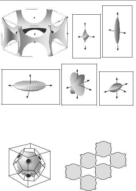
These are much more complicated than the alkali metals. They have two valence electrons per atom, but band overlapping causes the alkaline earths to form metals rather than insulators. Fig. 5.2 shows the Fermi surfaces for Mg. The case for sec- ond-zone holes has been called “Falicov’s Monster”. Examples of the alkaline earth metals include Be, Mg, Ca, Sr, and Ra. A nice discussion of this as well as other Fermi surfaces is given by Harrison [56, Chap. 3].
5.2.4 The Noble Metals (B)
The Fermi surface for the noble metals is typically more complicated than for the alkali metals. The Fermi surface of Cu is shown in Fig. 5.3. Other examples are Zn, Ag, and Au. Further information about Fermi surfaces is given in Table 5.1.
1 See Wigner and Huntington [5.32].
272 5 Metals, Alloys, and the Fermi Surface
H
A
L
H
K
Γ
Γ
K
M
A
L
M
K
H
(a)
(b)
(c)
M
A
M
H
H
K
K
H
A
H
A
M
M
M
(d)
(e)
(f)
Fig. 5.2. Fermi surfaces in magnesium based on the single OPW model: (a) second-zone holes, (b) first-zone holes, (c) third-zone electrons, (d) third-zone electrons, (e) third-zone electrons, (f) fourth-zone electrons. [Reprinted with permission from Ketterson JB and Stark RW, Physical Review, 156(3), 748 (1967). Copyright 1967 by the American Physical Society.]
(a)
(b)
Fig. 5.3. Sketch of the Fermi surface of Cu (a) in the first Brillouin zone, (b) in a cross Section of an extended zone representation
5.3 Experiments Related to the Fermi Surface (B)
273
Table 5.1. Summary of metals and Fermi surface
The Fermi energy EF is the highest filled electron energy at absolute zero. The Fermi surface is the locus of points in k space such that E(k) = EF.
Type of metal
Fermi surface
Comment
Free-electron gas
Sphere
Alkali (bcc)
Nearly spherical
Specimens hard to
(monovalent, Na, K, Rb, Cs)
work with
Alkaline earth (fcc)
See Fig. 5.2.
Can be complex
(Divalent, Be, Mg, Ca, Sr, Ba)
Noble
Distorted sphere makes con-
Specimens need to be
(monovalent, Cu Ag, Au)
tact with hexagonal faces –
pure and single crystal
complex in repeated zone
scheme. See Fig. 5.3.
Many more complex examples are discussed in Ashcroft and Mermin [21 Chap. 15]. Examples include tri (e.g. Al and tetravalent (e.g. Pb) metals, transition metals, rare earth metals, and semimetals (e.g. graphite).
There were many productive scientists connected with the study of Fermi surfaces, we mention only: A. B. Pippard, D. Schoenberg, A. V. Gold, and A. R. Mackintosh.
Experimental methods for studying the Fermi surface include the de Haas–van Alphen effect, the magnetoacoustic effect, ultrasonic attenuation, magnetoresistance, anomalous skin effect, cyclotron resonance, and size effects (see Ashcroft and Mermin [21 Chap. 14]. See also Pippard [5.24]. We briefly discuss some of these in Sect. 5.3.
5.3 Experiments Related to the Fermi Surface (B)
We will describe the de Haas–van Alphen effect in more detail in the next section. Under suitable conditions, if we measure the magnetic susceptibility of a metal as a function of external magnetic field, we find oscillations. Extreme cross-sections of the Fermi surface normal to the direction of the magnetic field are determined by the change of magnetic field that produces one oscillation. For similar physics reasons, we may also observe oscillations in the Hall effect, and thermal conductivity, among others.
We can also measure the dc electrical conductivity as a function of applied magnetic field as in magnetoresistance experiments. Under appropriate conditions, we may see an oscillatory change with the magnetic field as in the de Haas– -Schubnikov effect. Under other conditions, we may see a steady change of the conductivity with magnetic field. The interpretation of these experiments may be somewhat complex.
274 5 Metals, Alloys, and the Fermi Surface
In Chap. 6, we will discuss cyclotron resonance in semiconductors. As we will see then, cyclotron resonance involves absorption of energy from an alternating electric field by an electron that is circling about a magnetic field. In metals, due to skin-depth problems, we need to use the Azbel–Kanergeometry that places both the electric and magnetic fields parallel to the metallic surface. Cyclotron resonance provides a way of finding the effective mass m* appropriate to extremal sections of the Fermi surface. This can be used to extrapolate E(k) away from the Fermi surface.
Magnetoacoustic experiments can determine extremal dimensions of the Fermi surface normal to the plane formed by the ultrasonic wave and perpendicular magnetic field. It turns out that as we vary the magnetic field we find oscillations in the ultrasonic absorption. The oscillations depend on the wavelength of the ultrasonic waves. Proper interpretation gives the information indicated. Another technique for learning about the Fermi surface is the anomalous skin effect. We shall not discuss this technique here.
5.4 The de Haas–van Alphen effect (B)
The de Haas–van Alphen effect will be studied as an example of how experiments can be used to determine the Fermi surface and as an example of the wave-packet description of electrons. The most important factor in the de Haas–van Alphen effect involves the quantization of electron orbits in a constant magnetic field. Classically, the electrons revolve around the magnetic field with the cyclotron frequency
ωc = eB .
(5.17)
m
There may also be a translational motion along the direction of the field. Let τ be the mean time between collisions for the electrons, T be the temperature, and k be the Boltzmann constant.
In order for the de Haas–van Alphen effect to be detected, two conditions must be satisfied. First, despite scattering, the orbits must be well defined, or
ωcτ > 2π .
(5.18)
Second, the quantization of levels should not be smeared out by the thermal motion so
ωc > kT .
(5.19)
The energy difference between the quantized orbits is
ωc, and kT is the average
energy of thermal motion. To satisfy these conditions, we need large τ and large ωc, or high purity, low temperatures, and high magnetic fields.