4.5 The Boltzmann Equation and Electrical Conductivity |
245 |
|
|
If no collisions occurred, the r and k coordinates of every electron would evolve by the semiclassical equations of motion as will be shown (Sect. 6.1.2). That is:
vkσ = |
1 |
∂Ekσ |
, |
(4.114) |
|
∂k |
|
|
|
|
and |
|
|
|
|
k = Fext , |
|
(4.115) |
where F = Fext is the external force. Consider an electron having spin σ at r and k and time t started from r – vkσdt, k – Fdt/ at time t – dt. Conservation of the number of electrons then gives us:
fkσ (r,t)drtdkt = f(k −Fdt / )σ (r − vkσ dt ,t − dt)drt −dtdkt −dt . (4.116)
Liouville’s theorem then says that the electrons, which move by their equation of motion, preserve phase space volume. Thus, if there were no collisions:
fkσ (r,t) = f(k −Fdt / |
)σ (r − vkσ dt ,t − dt) . |
(4.117) |
Scattering due to collisions must be considered, so let |
|
Q(r, k,t) = |
∂f |
kσ |
|
(4.118) |
|
|
|
|
|
∂t |
collisions |
|
be the net change, due to collisions, in the number of electrons ( per dkdr/(2π)3) that get to r, k at time t. By expanding to first order in infinitesimals,
|
|
∂f |
kσ |
vkσ |
|
∂f |
kσ |
|
F |
|
|
∂f |
kσ |
|
fkσ (r,t) = |
fkσ (r,t) − dt |
|
+ |
|
|
+ |
|
+ Q(r,k,t)dt , |
|
|
|
|
|
|
∂r |
|
|
|
∂k |
|
|
|
|
∂t |
|
so |
|
|
|
|
|
|
|
|
|
|
|
|
|
|
|
|
|
Q(r,k,t) = |
∂fkσ |
|
vkσ + |
∂fkσ |
|
F + |
∂fkσ |
. |
|
∂r |
∂k |
|
|
|
|
|
|
|
|
|
|
|
|
|
∂t |
If the steady state is assumed, then
∂f∂ktσ = 0 .
Equation (4.120) may be the basic equation we need to solve, but it does us little good to write it down unless we can find useful expressions for Q. Evaluation of Q is by a detailed consideration of the scattering process. For many cases Q is determined by the scattering matrices as was discussed in Sects. 4.1 and 4.2. Even after Q is so determined, it is by no means a trivial problem to solve the Boltzmann integrodifferential (as it turns out to be) equation.
246 4 The Interaction of Electrons and Lattice Vibrations
4.5.2 Motivation for Solving the Boltzmann Differential Equation (B)
Before we begin discussing the Q details, it is worthwhile to give a little motivation for solving the Boltzmann differential equation. We will show how two important quantities can be calculated once the solution to the Boltzmann equation is known. It is also very useful to approximate Q by a phenomenological argument and then obtain solutions to (4.120). Both of these points will be discussed before we get into the rather serious problems that arise when we try to calculate Q from first principles.
Solutions to (4.120) allow us, from fkσ, to obtain the electric current density J, and the electronic flux of heat energy H. By definition of the distribution function, these two important quantities are given by
|
J = ∑σ ∫ (−e)vkσ fkσ |
|
dk |
|
, |
(4.122) |
|
(2π)3 |
|
|
|
|
|
H = ∑σ ∫ Ekσ vkσ fkσ |
|
dk |
. |
(4.123) |
|
|
(2π)3 |
|
|
|
|
|
Electrical conductivity σ and thermal conductivity κ 10 are defined by the relations
J = σE , |
(4.124) |
H = −κ T |
(4.125) |
(with a few additional restrictions as will be discussed, see, e.g., Sect. 4.6 and Table 4.5).
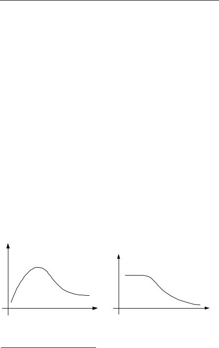
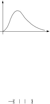
As long as we are this close, it is worthwhile to sketch the type of experimental results that are obtained for the transport coefficients κ and σ. In particular, it is useful to understand the particular form of the temperature dependences that are given in Fig. 4.7, Fig. 4.8, and Fig. 4.9. See Problems 4.2, 4.3, and 4.4.
Fig. 4.7. The thermal conductivity of a good metal (e.g. Na as a function of temperature)
Fig. 4.8. The electrical conductivity of a good metal (e.g. Na as a function of temperature)
10 See Table 4.5 for a more precise statement about what is held constant.
4.5 The Boltzmann Equation and Electrical Conductivity |
247 |
|
|
Fig. 4.9. The thermal conductivity of an insulator as a function of temperature, β θD/2
4.5.3 Scattering Processes and Q Details (B)
We now discuss the Q details. A typical situation in which we are interested is how to calculate the electron–phonon interaction and thus calculate the electrical resistivity. To begin with we consider how
is determined by the interactions. Let Pkσ, k′σ′ be the probability per unit time to scatter from the state k′σ′ to kσ. This is typically evaluated from the Golden rule of time-dependent perturbation theory (see Appendix E):
Pk′σ ′ = 2π |
kσ V k′σ′ 2 |
δ (E |
kσ |
− E |
k′σ ′ |
) . |
(4.126) |
kσ |
int |
|
|
|
|
The probability that there is an electron at r, k, σ available to be scattered is fkσ and (1 – fk′σ′) is the probability that k′σ′ can accept an electron (because it is empty).
For scattering out of kσ we have
∂f |
kσ |
|
= −∑ |
|
P ′ ′ |
f |
|
(1− f |
′ ′) . |
|
|
k′σ ′ |
kσ |
∂t |
c,out |
|
k σ ,kσ |
|
|
k σ |
|
|
|
|
|
|
|
By a similar argument for scattering into kσ, we have
∂f |
kσ |
|
= +∑ |
|
P |
′ ′ f |
′ ′(1− f |
|
) . |
|
|
k′σ ′ |
kσ |
∂t |
c,in |
|
kσ,k σ |
k σ |
|
|
|
|
|
|
|
|
Combining these two we have an expression for Q:
|
|
|
|
|
|
|
|
|
|
|
|
|
|
Q(r, k,t) = |
∂f |
kσ |
|
|
|
|
|
|
|
|
|
|
|
|
|
|
|
|
|
|
|
|
|
|
∂t |
c |
|
|
|
|
|
|
|
|
|
= ∑ |
k′σ ′ |
[P |
′ ′ f |
′ ′(1− f |
kσ |
) − P ′ ′ |
f |
kσ |
(1− f |
′ ′)] . |
|
|
|
kσ,k σ |
k σ |
k σ ,kσ |
|
|
k σ |
248 4 The Interaction of Electrons and Lattice Vibrations
This rate equation for fkσ is a type of Master equation [11, p. 190]. At equilibrium, the above must yield zero and we have the principle of detailed balance.
Pkσ,k′σ ′ fk0′σ ′(1− fk0σ ) = Pk′σ ′,kσ fk0σ (1− fk0′σ ′) .
Using the principle of detailed balance, we can write the rate equation as
Q(r, k,t) = |
∂f |
kσ |
|
|
|
|
|
|
|
|
|
|
|
|
|
|
|
|
|
|
|
|
|
|
|
|
|
|
|
|
|
|
|
|
|
|
|
|
|
|
∂t |
c |
|
|
|
|
|
|
|
|
|
|
|
|
|
|
) |
|
|
|
|
|
|
|
|
f |
k′σ ′ |
(1 |
− f |
kσ |
) |
|
f |
kσ |
(1 − f |
k′σ ′ |
= ∑ |
|
P ′ ′ |
|
f 0 |
(1 |
− f 0′ ′) |
|
|
|
|
− |
|
|
|
. |
|
|
f |
0′ ′ |
(1 |
− f |
|
) |
f |
|
(1 − f |
|
|
|
k′σ ′ |
k |
σ ,kσ |
kσ |
|
k σ |
|
0 |
|
0 |
0′ ′) |
|
|
|
|
|
|
|
|
|
|
k σ |
|
|
kσ |
|
|
|
kσ |
|
k σ |
|
|
We now define a quantity φkσ such that
|
|
|
|
0 |
|
|
∂fk0σ |
|
|
|
|
fkσ = |
fkσ |
−ϕkσ |
|
|
, |
|
|
|
|
∂Ekσ |
|
|
|
|
|
|
|
|
|
|
|
|
where |
|
|
|
|
|
|
|
|
|
|
fkσ |
= |
|
|
1 |
|
|
|
|
, |
|
exp[β(Ekσ |
− μ)] +1 |
|
|
|
|
(4.130)
(4.131)
(4.132)
(4.133)
with β = 1/kBT and fk0σ is the Fermi function. Noting that
|
|
|
|
|
∂fk0σ |
|
|
|
0 |
|
|
0 |
|
|
|
|
|
|
|
|
|
|
|
|
|
|
|
= −βfkσ (1 − fkσ ) , |
|
|
|
|
|
|
|
|
|
|
∂Ekσ |
|
|
|
|
|
|
|
|
|
|
|
|
|
|
|
|
|
|
|
|
|
|
|
|
we can show to linear order in φkσ that |
|
|
|
|
|
|
|
|
|
|
|
|
|
|
|
|
|
|
|
fk′σ ′ |
(1 − fkσ ) |
|
fkσ |
(1 |
− fk′σ ′) |
β(ϕk′σ ′ −ϕkσ ) = |
|
|
|
|
|
|
|
|
|
− |
|
|
|
|
|
. |
|
f |
0′ ′ |
(1 − f 0 |
) |
f 0 |
(1 |
|
|
|
|
|
|
|
|
|
|
|
− f 0′ ′) |
|
|
|
|
|
|
|
|
k σ |
|
|
kσ |
|
|
kσ |
|
k |
σ |
|
|
The Boltzmann transport equation can then be written in the form |
|
|
|
∂fkσ |
vkσ + |
∂fkσ |
|
F + |
|
∂fkσ |
= |
|
|
|
|
|
|
|
|
|
|
|
|
|
|
|
|
|
|
|
|
|
|
∂r |
|
|
∂k |
|
|
|
|
|
|
|
∂t |
|
|
|
|
|
|
|
|
|
|
β∑ |
|
|
P |
′ ′ |
|
f 0 (1− f |
0′ ′)(ϕ |
′ ′ −ϕ |
kσ |
) . |
|
|
|
k′σ ′ k σ ,kσ |
|
|
kσ |
k σ |
|
k σ |
|
|
|
Since the sums over k′ will be replaced by an integral, this is an integrodifferential equation.
Let us assume that in the Boltzmann equation, on the left-hand side, that there are small fields and temperature gradients so that fkσ can be replaced by its equilibrium value. Further, we will assume that fk0 σ characterizes local equilibrium in such a way that the spatial variation of fk0σ arises from the temperature and chemical potential (μ). Thus
∂fk0σ |
= |
∂fk0σ T + |
∂fk0σ μ = − |
(Ekσ − μ) |
T |
∂fk0σ |
− |
∂fk0σ |
μ . |
T |
|
|
∂r |
|
∂T |
∂μ |
|
∂Ekσ |
∂Ekσ |
4.5 The Boltzmann Equation and Electrical Conductivity |
249 |
|
|
We also use |
|
|
|
|
|
|
∂fkσ |
= |
vkσ |
∂fk0σ |
, |
(4.137) |
|
∂k |
|
|
|
|
∂Ekσ |
|
and assume an external electric field E so F = –eE. (The treatment of magnetic fields can be somewhat more complex, see, for example, Madelung [4.26, pp. 205 and following].)
We also replace the sums by integrals as follows:
|
∑k′σ ′ |
→ |
V |
∑σ′ ∫ dk′ . |
|
(2π)3 |
|
|
|
|
We assume steady-state conditions so ∂fkσ/∂t = 0. We thus write for the Boltzmann integrodifferential equation:
|
(E |
kσ |
− |
μ) |
|
|
|
∂f 0 |
|
|
1 |
|
|
|
∂f 0 |
|
|
− |
|
|
|
vkσ T |
kσ |
− e E + |
|
μ |
vkσ |
|
kσ |
|
|
|
|
T |
|
∂Ekσ |
e |
∂Ekσ |
|
|
|
|
V |
|
|
|
|
|
|
|
|
|
|
|
|
= |
|
|
∑ |
σ ′ ∫ |
dk′P ′ ′ |
f 0 |
(1 |
− f |
0′ ′)(ϕ |
′ ′ −ϕ |
kσ |
) (4.138) |
|
|
|
|
|
|
|
|
(2π)3 kT |
k σ ,kσ |
kσ |
|
k σ |
|
k σ |
|
≡∂fkσ .
∂t c
We now want to see under what conditions we can have a relaxation time. To this end we now assume elastic scattering. This can be approximated by electrons scattering from phonons if the phonon energies are negligible. In this case we write:
|
|
− |
V |
P |
|
f 0 |
(1− f 0 |
|
) =W (kσ, k′σ′)δ(E |
|
− E |
|
|
) , |
(4.139) |
|
|
|
|
|
|
|
|
|
|
|
(2π)3 k′σ ′,kσ |
kσ |
k′σ |
′ |
|
|
|
|
k′σ ′ |
|
kσ |
|
|
|
|
where the electron energies are given by Ekσ, so |
|
|
|
|
|
|
|
|
|
|
|
∂fkσ |
|
|
|
|
|
|
|
|
|
|
|
|
1 |
|
|
|
|
|
|
|
|
= −δf |
|
∑ ∫ |
dk′W (k |
′σ′, kσ) 1− δfk′σ |
′ |
|
|
δ(E |
|
|
− E |
|
). |
|
kσ |
0 |
|
|
k′σ ′ |
kσ |
∂t |
|
|
|
|
|
|
δfkσ |
|
∂Ekσ ) |
|
|
|
|
c |
|
|
|
σ ′ |
|
|
|
|
|
(∂fkσ |
|
|
|
|
(4.140) |
|
|
|
|
|
|
|
|
|
|
|
|
|
|
|
|
|
|
|
where δfkσ = fkσ – fk0σ We will also assume that the effect of external fields in the steady state causes a displacement of the Fermi distribution in k space. If the energy surface is also assumed to be spherical so E = E(k), with k equal to the magnitude of k, (and k′) we can write
fkσ |
= fk0σ |
− k c(E) |
∂fk0σ |
, |
(4.141) |
|
|
|
|
∂Ekσ |
|
250 4 The Interaction of Electrons and Lattice Vibrations
where c is a constant vector in the direction that f is displaced in k space. Thus
|
δfkσ |
= −k c(E) , |
|
∂fk0σ ∂Ekσ |
|
|
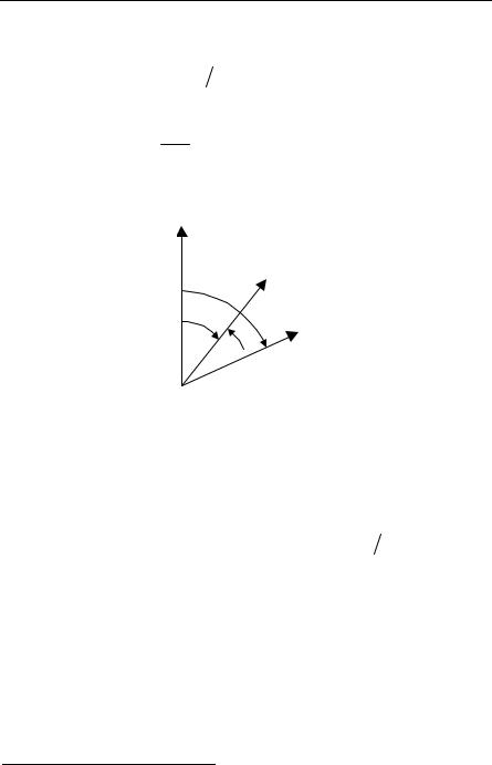
and from Fig. 4.10, we see we can write: |
|
cosΘ′ = cckk′ = sinθ sinΘ cosϕ′ + cosΘ cosθ . If we define a relaxation time by
k
k'
θ,ϕ
Θ ',ϕ '
Fig. 4.10. Orientation of the constant c vector with respect to k and k′ vectors
|
|
|
|
∂f |
|
|
= − |
δf |
kσ |
|
, |
|
|
(4.144) |
|
|
|
|
|
kσ |
|
|
|
|
|
|
|
|
|
∂t |
c |
|
τ(E) |
|
|
|
|
|
then |
|
|
|
|
|
|
|
|
|
|
|
|
|
|
|
|
1 |
= ∑ |
σ ′ ∫ |
dk′W (k′σ′, kσ)δ (E |
|
′ |
′ − E |
|
) |
(1− cosΘ) |
, (4.145) |
τ(E) |
|
|
|
|
|
|
|
|
|
k σ |
|
|
kσ |
|
∂fk0σ ∂Ekσ |
since the cos(φ′) vanishes on integration.
Expressions for ∂fkσ/∂t)c can be written down for various scattering processes. For example electron–phonon interactions can be sometimes evaluated as above using a relaxation-time approximation. Note if we were concerned with scattering of electrons from optical phonons, then in general their energies can not be neglected, and we would have neither an elastic scattering event, nor a relaxation-time approximation.11 In any case, the evaluation of Q is complex and further approximations are typically made.
An assumption that is often made in deriving an expression for electrical conductivity, as controlled by the electron–phonon interaction, is called the Bloch Ansatz. The Bloch Ansatz is the assumption that the phonon distribution remains
11For a discussion of how to treat such cases, see, for example, Howarth and Sondheimer [4.13].
4.5 The Boltzmann Equation and Electrical Conductivity |
251 |
|
|
in equilibrium even though the phonons scatter electrons and vice versa. By carrying through an analysis of electron scattering by phonons, using the approximations equivalent to the relaxation-time approximation (above), neglecting umklapp processes, and also making the Debye approximation for the phonons, Bloch evaluated the equilibrium resistivity of electrons as a function of temperature. He found that the electrical resistivity is approximated by
1 |
|
T |
5 |
θ |
|
/T |
x5dx |
|
|
|
|
|
|
∫ |
D |
|
|
. |
(4.146) |
|
|
|
(ex −1)(1− e−x ) |
σ |
|
θD |
0 |
|
|
|
|
This is called the Bloch–Gruneisen relation. In (4.146), θD is the Debye temperature. Note that (4.146) predicts the resistivity curve goes as T5 at low temperatures, and as T at higher temperatures.12 In (4.146), 1/σ is the resistivity ρ, and for real materials one should include a residual resistivity ρ0 as a further additive factor. The purity of the sample determines ρ0.
4.5.4The Relaxation-Time Approximate Solution of the Boltzmann Equation for Metals (B)
A phenomenological form of
= ∂f Q
∂t scatt
will be stated. We assume that (∂f/∂t)scatt (= ∂f/∂t)c) is proportional to the difference of f from its equilibrium f0 and is also proportional to the probability of
a collision 1/τ, where τ is the relaxation time, as in (4.144) and (4.145). Then
|
∂f |
|
f |
− f |
0 |
|
|
|
|
= − |
|
|
. |
(4.147) |
|
|
|
|
∂t scatt |
|
|
τ |
|
|
|
Integrating (4.147) gives |
|
|
|
|
|
|
|
|
f − f0 |
= Ae−t /τ , |
(4.148) |
which simply says that in the absence of external perturbations, any system will reach its equilibrium value when t becomes infinite. Equation (4.148) assumes that collisions will bring the system to equilibrium. This may be hard to prove, but it is physically very reasonable. There may be only a few cases where the assumption of a relaxation time is fully justified. To say more about this point requires a discussion of the Q details of the system. In (4.131), τ will be assumed to be a function of Ek only. A more drastic assumption would be that τ is a constant, and a less drastic assumption would be that τ is a function of k.
12As emphasized by Arajs [4.3], (4.146) should not be applied blindly with the expectation of good results in all metals (particularly for low temperature).
252 4 The Interaction of Electrons and Lattice Vibrations
With all of the above assumptions and assuming steady state, the Boltzmann differential equation is13
vk T |
∂fk |
− e(E + vk × B) vk |
∂fk |
= − |
fk − fk0 |
. |
(4.149) |
∂T |
∂Ek |
|
|
|
|
τ(Ek ) |
|
Since electrons are being considered, if we ignore the possibility of electron correlations, then fk0 is the Fermi–Dirac distribution function. (as in (4.154)).
In order to show the utility of (4.149), a calculation of the electrical conductivity using (4.149) will be made. We assume T = 0, B = 0, and E = Ezˆ . Then (4.149) reduces to
|
|
0 |
z |
∂fk |
|
|
|
fk = |
fk |
+ eτEvk |
|
. |
(4.150) |
|
∂Ek |
|
|
|
|
|
|
If we assume that there is only a small deviation from equilibrium, a first iteration yields
|
0 |
z |
∂fk0 |
|
fk = |
fk |
− eτEvk |
|
. |
(4.151) |
|
|
|
|
∂Ek |
|
Since there is no electrical current in equilibrium, substitution of (4.151) into (4.122) gives
|
e2 |
z |
2 |
|
∂fk0 |
|
3 |
|
|
J z = − |
|
∫ (vk ) |
|
τ |
|
Ed |
|
k . |
(4.152) |
4π 2 |
|
∂Ek |
|
|
|
|
|
|
|
|
|
If we have spherical symmetry in k space,
|
1 |
e2 |
2 |
∂fk0 |
|
3 |
|
|
J = − |
|
|
E∫ vkτ |
|
d |
|
k . |
(4.153) |
3 |
4π 2 |
∂Ek |
|
|
|
|
|
|
|
Since f k0 represents the value of the number of electrons, by our normalization (4.5.1)
fk0 = F the Fermi function. |
(4.154) |
At temperatures lower than several thousand degrees F 1 for Ek < EF and
F 0 for Ek > EF, and so |
|
|
∂F |
−δ (Ek − EF ) , |
(4.155) |
|
|
|
∂Ek |
|
13Equation (4.149) is the same as (4.138) and (4.145) with μ = 0 and B = 0. These are typical conditions for metals, although not necessarily for semiconductors.
4.6 Transport Coefficients |
253 |
|
|
where δ is the Dirac delta function and EF is the Fermi energy. Now since a volume in k-space may be written as
d3k = |
|
dSdE |
= dSdE , |
(4.156) |
|
k E |
|
|
vk |
|
where S is a surface of constant energy, (4.153), (4.154), (4.155), and (4.156) imply
J = |
e2E |
|
∫ [∫ vkτδ(Ek − EF )dE]dS . |
(4.157) |
|
|
12π3 |
|
|
|
|
Using Ek = 2k2/2m, (4.157) becomes |
|
|
|
J = |
|
e2E |
(vkF )(τF )4πkF2 , |
(4.158) |
|
12π3 |
|
|
|
|
where the subscript F means that the function is to be evaluated at the Fermi energy. If n is the number of conduction electrons per unit volume, then
|
1 |
|
∫ Fd |
3 |
|
4π |
3 |
1 |
|
|
n = |
|
|
|
k = |
|
kF |
|
. |
(4.159) |
4π |
3 |
|
3 |
4π3 |
|
|
|
|
|
|
|
Combining (4.158) and (4.159), we find that
J = ne2EτF |
=σE |
or σ = ne2τF . |
(4.160) |
m |
|
m |
|
This is (3.220) that was derived earlier. Now it is clear that all pertinent quantities are to be evaluated at the Fermi energy. There are several general techniques for solving the Boltzmann equation, for example the variation principle. The book by Ziman can be consulted [99, p275ff].
4.6 Transport Coefficients
As mentioned, if we have no magnetic field (in the presence of a magnetic field, several other characteristic effects besides those mentioned below are of importance [4.26, p 205] and [73]), then the approximate Boltzmann differential equation is (in the relaxation-time approximation)
|
|
|
0 |
|
|
0 |
|
|
0 |
|
|
vk |
|
− T |
∂fk |
+ eE |
∂fk |
|
= |
fk − fk |
. |
(4.161) |
|
∂T |
∂E |
|
|
τ |
|
|
|
|
|
|
|
k |
|
|
|
|
Using the definitions of J and H in terms of the distribution function ((4.122) and (4.123)), and using (4.161), we have
J = aE + b T , |
(4.162) |
H = cE + d T . |
(4.163) |
254 4 The Interaction of Electrons and Lattice Vibrations
For cubic crystals a, b, c, and d are scalars. Equations (4.162) and (4.163) are more general than their derivation based on (4.161) might suggest. The equations must be valid for sufficiently small E and T. This is seen by a Taylor series expansion and by the fact that J and H must vanish when E and T vanish. The point of this Section will be to show how experiments determine a, b, c, and d for materials in which electrons carry both heat and electricity.
4.6.1 The Electrical Conductivity (B)
The electrical conductivity measurement is the simplest of all. We simply setT = 0 and measure the electrical current. Equation (4.162) becomes J = aE, and so we obtain a = σ.
4.6.2 The Peltier Coefficient (B)
This is also an easy measurement to describe. We use the same experimental setup as for electrical conductivity, but now we measure the heat current. Equation (4.163) becomes
|
H = cE = c |
J |
= |
c |
J . |
(4.164) |
|
σ |
a |
|
|
|
|
|
The Peltier coefficient is the heat current per unit electrical current and so it is given by Π = c/a.
4.6.3 The Thermal Conductivity (B)
This is just a little more complicated than the above, because we usually do the thermal conductivity measurements with no electrical current rather than no electrical field. By the definition of thermal conductivity and (4.163), we obtain
K = − |
|
|
H |
|
|
= − |
|
|
cE + d T |
|
|
. |
(4.165) |
|
|
|
|
|
|
|
|
|
|
|
|
|
|
|
|
|
T |
|
|
|
T |
|
|
|
Using (4.162) with no electrical current, we have
|
E = − |
b |
T . |
(4.166) |
|
a |
|
|
|
|
|
The thermal conductivity is then given by |
|
|
|
K = −d + cb . |
(4.167) |
|
|
|
a |
|
We might expect the thermal conductivity to be −d, but we must remember that we required there to be no electrical current. This causes an electric field to appear, which tends to reduce the heat current.