Patterson, Bailey - Solid State Physics Introduction to theory

5.8 Electromigration (EE, MS) 285

the momentum of the electron before and after collision, and pa and Pa be the momentum of the ion before and after. By momentum and energy conservation we have:

where V0 is the magnitude of the potential hole the ion is in before collision, and m and ma are the masses of the electron and the ion, respectively. Solving for Pa and P in terms of pa and p, retaining only the physically significant roots and assuming m << ma:

In order to move the ion, the electron’s kinetic energy must be greater than V0 as perhaps is obvious. However, the process by which ions are started in motion is surely more complicated than this description, and other phenomena, such as the presence of vacancies are involved. Indeed, electromigration is often thought to occur along grain boundaries.

For the simplest model, we may as well start by setting V0 equal to zero. This makes the collisions elastic. We will assume that the ions are pushed along by the electron wind, but there are other forces that cancel out the wind force, so that the flow is in steady state. The relevant conservation equations become:

Pa = pa + 2 p , P = −p.

We will consider motion in one dimension only. The ions drift along with a momentum pa. The electrons move back and forth between the drifting ions with momentum p. We assume the electron’s velocity is so great that the ions are stationary in comparison. Assume the electric field points along the −x-axis. Electrons moving to the right collide and increase the momentum of the ions, and those moving to the left decrease their momentum. Because of the action of the electric field, electrons moving to the right have more momentum so the net effect is a small increase in the momentum of the ions (which, as mentioned, is removed by other effects to produce a steady-state drift). If E is the electric field, then in time τ, (the time taken for electrons to move between ions), an electron of charge −e gains momentum

if it moves against the field, and it loses a similar amount of momentum if it goes in the opposite direction. Assume the electrons have momentum p when they are

and the mass of the star is, neglecting electron mass and assuming the neutron mass equals the proton mass (mp) and that there are the same number of each

We now want to work out the conditions for equilibrium. Without gravity, the work to compress the electrons is

Gravitational energy is approximately (with α = 1)

If R is the equilibrium radius of the star, since gravitational self-energy plus work to compress = 0, we have

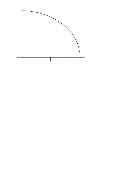
and this result is good for small R (and large xF). A more precise derivation pre-

dicts M0 1.4Msun. Thus, there is no white dwarf star with mass M ≥ M0 Msun. See Fig. 5.8. M0 is known as the mass for the Chandrasekhar limit. When the mass

is greater than M0, the Pauli principle is not sufficient to support the star against gravitational collapse. It may then become a neutron star or even a black hole, depending upon the mass.

Problems 291

Chromium Chrome plated over nickel to produce an attractive finish is a major use. It is also used in alloy steels to increase hardness.

Gold Along with silver and platinum, gold is one of the precious metals. Its use as a semiconductor connection in silicon is important.

Titanium Much used in the aircraft industry because of the strength and lightness of its alloys.

Tungsten Has the highest melting point of any metal and is used in steels, as filaments in light bulbs and in tungsten carbide. The hardest known metal.

Problems

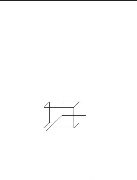
5.1For the Hall effect (metals-electrons only), find the Hall coefficient, the effec-

tive conductance jx/Ex, and σyx. For high magnetic fields, relate σyx to the Hall coefficient. Assume the following geometry:

y, Ey

jy

z, Bz

Reference can be made to Sect. 6.1.5 for the definition of the Hall effect.

5.2(a) A twodimensional metal has one atom of valence one in a simple rectan-

gular primitive cell a = 2, b = 4 (units of angstroms). Draw the First Brillouin zone and give dimensions in cm–1.

(b)Calculate the areal density of electrons for which the free electron Fermi surface first touches the Brillouin zone boundary.

5.3For highly relativistic conditions within a white dwarf star, derive the rela-

tionship for pressure p0 as a function of mass M and radius R using p0 =

− ∂E0/∂V.

5.4Consider the current due to metal-insulator-metal tunneling. Set up an expression for calculating this current. Do not necessarily assume zero temperature. See, e.g., Duke [5.6].

5.5Derive (5.37).

6 Semiconductors

Starting with the development of the transistor by Bardeen, Brattain, and Shockley in 1947, the technology of semiconductors has exploded. With the creation of integrated circuits and chips, semiconductor devices have penetrated into large parts of our lives. The modern desktop or laptop computer would be unthinkable without microelectronic semiconductor devices, and so would a myriad of other devices.

Recalling the band theory of Chap. 3, one could call a semiconductor a narrowgap insulator in the sense that its energy gap between the highest filled band (the valence band) and the lowest unfilled band (the conduction band) is typically of the order of one electron volt. The electrical conductivity of a semiconductor is consequently typically much less than that of a metal.

The purity of a semiconductor is very important and controlled doping is used to vary the electrical properties. As we will discuss, donor impurities are added to increase the number of electrons and acceptors are added to increase the number of holes (which are caused by the absence of electrons in states normally electron occupied – and as discussed later in the chapter, holes act as positive charges). Donors are impurities that become positively ionized by contributing an electron to the conduction band, while acceptors become negatively ionized by accepting electrons from the valence band. The electrons and holes are thermally activated and in a temperature range in which the charged carriers contributed by the impurities dominate, the semiconductor is said to be in the extrinsic temperature range, otherwise it is said to be intrinsic. Over a certain temperature range, donors can add electrons to the conduction band (and acceptors can add holes to the valence band) as temperature is increased. This can cause the electrical resistivity to decrease with increasing temperature giving a negative coefficient of resistance. This is to be contrasted with the opposite behavior in metals. For group IV semiconductors (Si, Ge) typical donors come from column V of the periodic table (P, As, Sb) and typical acceptors from column III (B, Al, Ga, In).

Semiconductors tend to be bonded tetrahedrally and covalently, although binary semiconductors may have polar, as well as covalent character. The simplest semiconductors are the nonpolar semiconductors from column 4 of the Periodic Table: Si and Ge. Compound III-V semiconductors are represented by, e.g., InSb and GaAs while II-VI semiconductors are represented by, e.g., CdS and CdSe. The pseudobinary compound Hg(1–x)Cd(x)Te is an important narrow gap semiconductor whose gap can be varied with concentration x and it is used as an infrared detector. There are several other pseudobinary alloys of technical importance as well.

Table 6.1. Important properties of representative semiconductors (A)

* Adapted from Sze SM (ed), Modern Semiconductor Device Physics, Copyright © 1998, John Wiley & Sons, Inc, New York, pp. 537-540. This material is used by permission of John Wiley & Sons, Inc.

Table 6.2. Important properties of representative semiconductors (B)

*ml is longitudinal, mt is transverse.

**mlh is light hole, mhh is heavy hole.

Adapted from Sze SM (ed), Modern Semiconductor Device Physics, Copyright © 1998, John Wiley & Sons, Inc, New York, pp. 537-540. This material is used by permission of John Wiley & Sons, Inc.