Eh (kh ) = −Ee (−ke ) ,
Eh (kh ) = −Ee (ke ) .
where Σ′ k means the sum over k omitting ke. Thus, we have, assuming symmetric bands with Ee(ke) = Ee(−ke):
(6.58)
or
(6.59)
Notice also, since
|
dke |
= −e(E + ve × B) , |
(6.60) |
|
dt |
|
|
|
with qh = +e, kh = −ke and ve = vh, we have
|
dkh |
= +e(E + vh × B) , |
(6.61) |
|
dt |
|
|
|
as expected. Now, since
ve = |
1 ∂Ee (ke ) = |
1 ∂ (−Eh (kh )) |
= |
1 ∂Eh , |
|
|
∂ (ke ) |
|
|
|
|
∂ (−kh ) |
|
∂kh |
and since ve = vh, then |
|
|
|
|
|
|
|
|
|
|
|
|
|
|
|
|
|
vh |
= |
|
1 |
∂Eh . |
|
|
|
|
|
|
|
|
|
|
|
|
|
|
|
|
|
∂kh |
|
|
Now, |
|
|
|
|
|
|
|
|
|
|
|
|
|
dvh = |
1 |
∂ 2Eh |
dkh = |
1 |
∂ 2Eh F . |
|
|
|
dt |
|
|
∂kh2 |
|
dt |
|
2 ∂kh2 |
h |
|
|
|
|
|
|
Defining the hole effective mass as
|
|
1 |
|
= |
1 |
∂ |
|
2E |
h , |
|
|
(6.65) |
|
|
|
mh |
|
|
|
|
|
|
|
|
|
|
|
|
|
|
2 |
|
∂kh2 |
|
|
|
we see |
|
|
|
|
|
|
|
|
|
|
|
|
|
|
|
|
|
|
1 |
= − |
|
1 |
|
|
∂ 2E |
e |
|
= − |
1 |
, |
(6.66) |
|
m |
|
|
2 ∂ (−k |
|
|
|
m |
|
|
|
|
|
e |
)2 |
|
|
|
|
|
h |
|
|
|
|
|
|
|
|
|
|
|
|
e |
|
|
or |
|
|
|
|
|
|
|
|
|
|
|
|
|
|
|
|
|
|
|
|
|
|
m = −m . |
|
|
|
(6.67) |
|
|
|
|
|
|
e |
|
|
|
|
h |
|
|
|
|
Notice that if Ee = Ak2, where A is constant then me* > 0, whereas if Ee = −Ak2, then mh* = −me* > 0, and concave down bands have negative electron masses but positive hole masses. Later we note that electrons and holes may interact so as to form excitons (Sect. 10.7, Exciton Absorption).

6.1 Electron Motion 307
6.1.4 Conductivity and Mobility in Semiconductors (B)
Current can be produced in semiconductors by, e.g., potential gradients (electric fields) or concentration gradients. We now discuss this.
We assume, as is usually the case, that the lifetime of the carriers is very long compared to the mean time between collisions. We also assume a Drude model with a unique collision or relaxation time τ. A more rigorous presentation can be made by using the Boltzmann equation where in effect we assume τ = τ(E). A consequence of doing this is mentioned in (6.102).
We are actually using a semiclassical Drude model where the effect of the lattice is taken into account by using an effective mass, derived from the band structure, and we treat the carriers classically except perhaps when we try to estimate their scattering. As already mentioned, to regard the carriers classically we must think of packets of Bloch waves representing them. These wave packets are large compared to the size of a unit cell and thus the field we consider must vary slowly in space. An applied field also must have a frequency much less than the bandgap over in order to avoid band transitions.
We consider current due to drift in an electric field. Let v be the drift velocity of electrons, m* be their effective mass, and τ be a relaxation time that characterizes the friction drag on the electrons. In an electric field E, we can write (for e > 0)
m dv = − m v − eE . dt τ
Thus in the steady state
v = − eτE . m
If n is the number of electrons per unit volume with drift velocity v, then the current density is
j = −nev . |
(6.70) |
Combining the last two equations gives |
|
2 |
|
j = ne τ*E . |
(6.71) |
m |
|
Thus, the electrical conductivity σ, defined by j/E, is given by |
|
ne2τ |
|
σ = m* . |
(6.72) |
3 The electrical mobility is the magnitude of the drift velocity per unit electric field |v/E|, so
3We have already derived this, see, e.g., (3.214) where effective mass was not used and in (4.160) where again the m used should be effective mass and τ is more precisely evaluated at the Fermi energy.
Notice that the mobility measures the scattering, while the electrical conductivity measures both the scattering and the electron concentration. Combining the last two equations, we can write
If we have both electrons (e) and holes (h) with concentration n and p, then
where
μe = eτe , me
and
μh = eτh . mh
The drift current density Jd can be written either as
Jd = −neve + pevh ,
or
Jd = [(neμe ) + ( peμh )]E .
(6.76)
(6.77)
(6.78)
(6.79)
As mentioned, in semiconductors we can also have current due to concentration gradients. By Fick’s Law, the diffusion number current is negatively proportional to the concentration gradient with the proportionality constant equal to the diffusion constant. Multiplying by the charge gives the electrical current density. Thus,
J |
e, diffusion |
= eD |
dn |
|
(6.80) |
|
|
|
e |
|
dx |
|
|
J |
h, diffusion |
= −eD |
|
dp |
. |
(6.81) |
|
dx |
|
|
h |
|
|
|
For both drift and diffusion currents, the electronic current density is |
|
J |
e |
= μ |
e |
enE + eD |
dn |
, |
(6.82) |
|
|
|
|
|
|
|
|
|
e dx |
|
|
and the hole current density is |
|
|
|
|
|
|
|
|
|
|
|
|
|
|
J |
h |
= μ |
h |
epE − eD |
|
dp |
. |
(6.83) |
|
|
|
|
|
|
|
h dx |
|
|
In both cases, the diffusion constant can be related to the mobility by the Einstein relationship (valid for both Drude and Boltzmann models)
eDe = μekT , |
(6.84) |
eDh = μhkT . |
(6.85) |
6.1.5Drift of Carriers in Electric and Magnetic Fields: The Hall Effect (B)
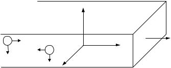
The Hall effect is the production of a transverse voltage (a voltage change along the “y direction”) due to a transverse B-field (in the “z direction”) with current flowing in the “x direction.” It is useful for determining information on the sign and concentration of carriers. See Fig. 6.4.
If the collisional force is described by a relaxation time τ,
m dv |
= −e(E + v × B) − m |
v |
, |
(6.86) |
|
e dt |
e τe |
|
where v is the drift velocity. We treat the steady state with dv/dt = 0. The magnetic field is assumed to be in the z direction and we define
ωe = eB , the cyclotron frequency, |
(6.87) |
me |
|
|
|
|
and |
|
|
|
|
μe |
= |
eτe |
, the mobility. |
(6.88) |
|
|
|
me |
|
For electrons, from (6.86) we can write the components of drift velocity as (steady state)
ve |
= −μ |
e |
E |
x |
−ω τ |
ve |
, |
(6.89) |
x |
|
|
e e |
y |
|
|
ve |
= −μ |
e |
E |
y |
+ω τ |
ve |
, |
(6.90) |
y |
|
|
e e |
x |
|
|
y
h |
v |
|
E |
|
x |
|
v |
e |
|
|
Force |
|
|
z, B |
|
|
Force |
|
|
|
Fig. 6.4. Geometry for the Hall effect

where vez = 0, since Ez = 0. With similar definitions, the equations for holes become
vh = +μ |
h |
E |
x |
+ω τ |
vh , |
(6.91) |
x |
|
h h |
y |
|
vh = +μ |
h |
E |
y |
−ω τ |
vh . |
(6.92) |
y |
|
h h |
x |
|
Due to the electric field in the x direction, the current is |
|
jx = −nevxe + pevxh . |
(6.93) |
Because of the magnetic field in the z direction, there are forces also in the y direction, which end up creating an electric field Ey in that direction. The Hall coefficient is defined as
H jx B
Equations (6.89) and (6.90) can be solved for the electrons drift velocity and (6.91) and (6.92) for the hole’s drift velocity. We assume weak magnetic fields and neglect terms of order ω2e and ωh2 , since ωe and ωh are proportional to the magnetic field. This is equivalent to neglecting magnetoresistance, i.e. the variation with resistance in a magnetic field. It can be shown that for carriers of two types if we retain terms of second order then we have a magnetoresistance. So far we have not considered a distribution of velocities as in the Boltzmann approach. Combining these assumptions, we get
vxe = −μeEx + μeωeτeEy ,
vxh = +μh Ex + μhωhτh Ey ,
vey = −μeEy − μeωeτeEx ,
vhy = +μh Ey − μhωhτh Ex .
Since there is no net current in the y direction,
jy = −nevey + pevhy = 0 . Substituting (6.97) and (6.98) into (6.99) gives
Ex = −Ey |
nμe + pμh |
|
|
|
|
. |
nμ ω τ |
− pμ |
h |
ω τ |
|
e e e |
|
h h |
(6.95)
(6.96)
(6.97)
(6.98)
(6.99)
(6.100)
Putting (6.95) and (6.96) into jx, using (6.100) and putting the results into RH, we find
|
|
|
|
|
|
R |
= 1 |
p − nb2 |
, |
(6.101) |
|
H |
e ( p + nb)2 |
|
|
|
|
|
|
where b = μe/μh. Note if p = 0, RH = −1/ne and if n = 0, RH = +1/pe. Both the sign and concentration of carriers are included in the Hall coefficient. As noted, this development did not take into account that the carrier would have a velocity distribution. If a Boltzmann distribution is assumed,
|
1 |
|
p − nb2 |
|
|
RH = r |
|
|
|
, |
(6.102) |
|
( p + nb)2 |
e |
|
|
|
where r depends on the way the electrons are scattered (different scattering mechanisms give different r).
The Hall effect is further discussed in Sects. 12.6 and 12.7, where peculiar effects involved in the quantum Hall effect are dealt with. The Hall effect can be used as a sensor of magnetic fields since it is proportional to the magnetic field for fixed currents.
6.1.6 Cyclotron Resonance (A)
Cyclotron resonance is the absorption of electromagnetic energy by electrons in a magnetic field at multiples of the cyclotron frequency. It was predicted by Dorfmann and Dingel and experimentally demonstrated by Kittel all in the early 1950s.
In this section, we discuss cyclotron resonance only in semiconductors. As we will see, this is a good way to determine effective masses but few carriers are naturally excited so external illumination may be needed to enhance carrier concentration (see further comments at the end of this section). Metals have plenty of carriers but skin-depth effects limit cyclotron resonance to those electrons near the surface (as discussed in Sect. 5.4).
We work on the case for Si. See also, e.g. [6.33, pp. 78-83]. We impose a magnetic field and seek the natural frequencies of oscillatory motion. Cyclotron resonance absorption will occur when an electric field with polarization in the plane of motion has a frequency equal to the frequency of oscillatory motion due to the magnetic field. We first look at motion for the energy lobes along the kz-axis (see Si in Fig. 6.6). The energy ellipsoids are not centered at the origin. Thus, the two constant energy ellipsoids along the kz-axis can be written
2 |
k 2 + k 2 |
|
|
|
|
x |
y |
|
E = 2 |
|
|
m |
+ |
|
|
|
|
T |
|
(k |
z |
− k |
0 |
)2 |
|
|
|
|
|
|
. |
(6.103) |
|
|
m |
|
|
|
|
|
L |
|
|
|
|
|
|
|
|
|
|
|
The shape of the ellipsoid determines the effective mass (T for transverse, L for longitudinal) in (6.103). The star on the effective mass is eliminated for simplicity. The velocity is given by
so
vx = kx mT
|
|
|
|
|
|
|
vy = |
k y |
|
|
mT |
|
|
|
|
vz = |
(kz − k0 ) |
. |
|
|
|
|
|
mL |
The equation of motion for charge q is
ddkt = qv × B .
(6.105)
(6.106)
(6.107)
(6.108)
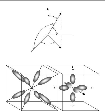
Writing out the three components of this equation, and substituting the equations for the velocity, we find with (see Fig. 6.5)
|
|
|
|
|
|
|
Bx = B sinθ cosφ , |
|
|
|
|
|
|
|
|
|
|
|
By = B sinθ sinφ , |
|
|
|
|
|
|
|
|
|
|
|
|
|
Bz = B cosθ , |
|
|
|
|
|
dkx |
k y |
cosθ |
|
(kz − k0 ) |
|
|
|
|
|
|
|
|
= qB |
|
|
|
|
− |
|
|
|
sinθ sinφ |
, |
|
dt |
mT |
mL |
|
|
|
|
|
|
|
dk y |
(kz |
− k0 ) |
|
|
|
|
|
kx |
|
|
|
|
|
|
= qB |
|
|
|
|
|
|
sinθ cosφ − |
|
cosθ |
, |
|
dt |
|
|
mL |
mT |
|
|
|
|
|
|
|
|
|
|
dkz |
kx |
|
|
|
|
|
k y |
|
|
|
|
|
|
= qB |
|
|
sinθ sinφ − |
|
|
sinθ cosφ . |
|
dt |
|
m |
|
m |
|
|
|
|
|
T |
|
|
|
|
|
T |
|
|
|
|
Seeking solutions of the form
kx = A1 exp(iωt) , k y = A2 exp(iωt) ,
(kz − k0 ) = A3 exp(iωt) , and defining a, b, c, and γ for convenience,
a = qB cosθ , mT
b = qB sinθ sinφ , mL
(6.109)
(6.110)
(6.111)
(6.112)
(6.113)
(6.114)
(6.115)
(6.116)
(6.117)
(6.118)
(6.119)
|
|
|
|
|
6.1 Electron Motion 313 |
|
|
|
|
c = |
qB |
sinθ cosφ , |
(6.120) |
|
|
m |
|
|
|
|
|
L |
|
|
|
|
|
γ |
= mL |
, |
(6.121) |
|
|
|
m |
|
|
|
|
|
T |
|
|
we can express (6.112), (6.113), and (6.114) in the matrix form
iω |
− a |
b a |
|
|
|
a |
iω |
|
|
= 0 . |
(6.122) |
|
− c b |
|
|
|
|
|
|
|
−bγ γc |
iω c |
|
|
Setting the determinant of the coefficient matrix equal to zero gives three solutions for ω,
ω = 0 , |
(6.123) |
and |
|
ω2 = a2 +γ (b2 + c2 ) . |
(6.124) |
After simplification, the nonzero frequency solution (6.124) can be written:
ω |
2 |
= (qB) |
2 |
cos2 θ |
+ |
sin2 θ |
(6.125) |
|
|
|
m2 |
. |
|
|
|
|
|
|
mLmT |
|
|
|
|
|
|
T |
|
|
|
Since we have two other sets of lobes in the electronic wave function in Si (along the x-axis and along the y-axis), we have two other sets of frequencies that can be obtained by substituting θx and θy for θ (Fig. 6.5 and Fig. 6.6).
Note from Fig. 6.5
cosθx = |
|
B i |
|
= sinθ cosφ |
(6.126) |
|
B |
|
|
|
|
|
cosθy = |
B j |
|
= sinθ sinφ . |
(6.127) |
|
B |
|
|
|
|
|
|
Thus, the three resonance frequencies can be determined. For the (energy) lobes along the z-axis, we have found
ω |
2 |
= (qB) |
2 |
cos2 |
θ |
+ |
sin2 θ |
z |
|
|
m2 |
|
. |
|
|
|
|
|
|
mLmT |
|
|
|
|
|
T |
|
|
|
For the lobes along the x-axis, replace θ with θx and get
ω |
2 |
= (qB) |
2 |
sin2 |
θ cos2 φ |
+ |
1−sin2 θ cos2 φ |
x |
|
|
m2 |
mLmT |
, |
|
|
|
|
|
|
|
|
|
|
|
T |
|
|
|
and for the lobes along the y-axis, replace θ with θy and get
ω |
2 |
= (qB) |
2 |
sin2 |
θ sin2 φ |
+ |
1−sin2 θ sin2 φ |
y |
|
|
m2 |
mLmT |
. |
|
|
|
|
|
|
|
|
|
|
|
T |
|
|
|
z
B
θ
θx θy 
 y
y
φ
x
Fig. 6.5. Definition of angles used for cyclotron-resonance discussion
 ky
ky
kx
Fig. 6.6. Constant energy ellipsoids in Ge and Si. From Ziman JM, Electrons and Phonons: The Theory of Transport Phenomena in Solids, Clarendon Press, Oxford (1960). By permission of Oxford University Press
In general, then we get three resonance frequencies. Obviously, for certain directions of B, some or all of these frequencies may become degenerate.
Several comments:
1.When mL = mT, these frequencies reduce to the cyclotron frequency ωc = qB/m.
2.In general, one will have to illuminate the sample to produce enough electrons and holes to detect the absorption, as with laser illumination.
3.In order to see the absorption, one wants collisions to be rare. If τ is the mean
time between collisions, we then require ωcτ > 1 or low temperatures, high purity, and high magnetic fields are required.
4.The resonant frequencies can be used to determine the longitudinal and transverse effective mass mL, mT.
5.Extremal orbits, with high density of states, are most important for effective absorption.
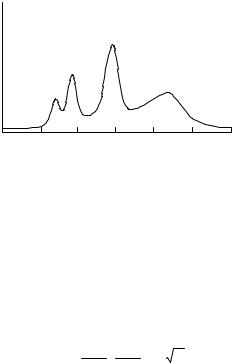
Some classic cyclotron resonance results obtained at Berkeley in 1955 by Dresselhaus, Kip, and Kittel are sketched in Fig. 6.7. See also the Section below “Power Absorption in Cyclotron Resonance.”
|
Silicon |
Electrons |
|
|
|
Absorption(arb.units) |
Lightholes |
Electrons |
Heavyholes |
|
|
0 |
1.0 |
2.0 |
3.0 |
4.0 |
5.0 |
6.0 |
Magnetic flux density B (kG)
Fig. 6.7. Sketch of cyclotron resonance for silicon. (near 24×103 Mc/s and 4 K, B at 30° with [100] and in (110) plane). Adapted from Dresselhaus, Kip and Kittel [6.11]
Density of States Effective Electron Masses for Si (A)
We can now generalize the concept of density of states effective mass so as to extend the use of equations like (6.4). For Si, we relate the transverse and longitudinal effective masses to the density of states effective mass. See “Density of States for Effective Hole Masses” in Sect. 6.2.1 for light and heavy hole effective masses. For electrons in the conduction band we have used the density of states.
D(E) = |
1 |
|
|
2m 3 / 2 |
E . |
(6.131) |
|
2 |
|
e |
|
2π |
|
2 |
|
|
|
|
|
|
|
|
|
|
This can be derived from |
|
|
|
|
|
|
|
D(E) = dn(E) |
= dn(E) |
dVk |
, |
|
dE |
|
|
dE |
|
dV |
|
|
|
|
|
|
k |
|
|
|