5.4 The de Haas–van Alphen effect (B) 275
We now consider the motions of the electrons in a magnetic field. For electrons in a magnetic field B, we can write (e > 0, see Sect. 6.1.2)
F = k = −e(v × B) , |
(5.20) |
and taking magnitudes |
|
|
|
dk = |
eB |
1 |
(5.21) |
|
v dt , |
where v1 is the component of velocity perpendicular to B and F.
It will take an electron the same length of time to complete a cycle of motion in real space as in k-space. Therefore, for the period of the orbit, we can write
T = |
2π = ∫ dt = |
|
∫ |
dk . |
(5.22) |
|
ωc |
eB |
|
v1 |
|
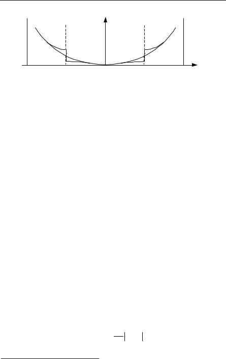
Since the force is perpendicular to the velocity of the electron, the constant magnetic field cannot change the energy of the electron. Therefore, in k-space, the electron must stay on the same constant energy surface. Only electrons near the Fermi surface will be important for most effects, so let us limit our discussion to these. That the motion must be along the Fermi surface follows not only from the fact that the motion must be at constant energy, but that dk is perpendicular to
because kE(k) is perpendicular to constant-energy surfaces. Equation (5.23) is derived in Sect. 6.1.2. The orbit in k-space is confined to the intersection of the Fermi surface and a plane perpendicular to the magnetic field.
In order to consider the de Haas–van Alphen effect, we need to relate the energy of the electron to the area of its orbit in k-space. We do this by considering
two orbits in k-space, which differ in energy by the small amount |
E. |
v = |
1 |
|
E |
, |
(5.24) |
|
|
|
|
|
k |
|
where v is the component of electron velocity perpendicular to the energy surface. From Fig. 5.4, note
v1 = v sinθ = |
1 |
|
|
E |
sinθ = |
1 |
|
|
|
E |
|
= |
1 |
|
E |
. |
(5.25) |
|
|
|
|
|
|
k sinθ |
|
|
|
|
|
|
|
|
|
|
|
k |
|
|
|
|
|
|
|
|
k1 |
|
Therefore, |
|
|
|
|
|
|
|
|
|
|
|
|
|
|
|
|
|
|
|
|
|
|
|
|
2π |
= |
|
|
∫ |
|
|
dk |
= |
2 |
|
1 ∫ |
k1 dk , |
|
|
(5.26) |
|
|
|
1 |
|
|
|
|
|
|
ω |
|
eB |
|
|
|
eB |
|
|
|
c |
|
|
|
E |
1 |
|
|
E |
|
|
|
|
|
|
|
|
|
|
|
|
|
|
|
k |
|
|
|
|
|
|
|
|
|
|
|
|
276 5 Metals, Alloys, and the Fermi Surface
B
k
Fig. 5.4. Constant-energy surfaces for the de Haas–van Alphen effect
and
2π |
= |
2 |
|
A |
, |
(5.27) |
|
|
eB |
E |
ωc |
|
|
|
where A is the area between the two Fermi surfaces in the plane perpendicular to B. This result was first obtained by Onsager in 1952 [5.20].
Recall that we have already found that the energy levels of an electron in a magnetic field (in the z direction) are given by (3.201)
|
|
|
|
|
1 |
|
|
2k 2 |
|
E |
n,kz |
= ω |
c |
n + |
|
|
+ |
z |
. |
(5.28) |
|
|
|
|
|
2 |
|
|
2m |
|
|
|
|
|
|
|
This equation tells us that the difference in energy between different orbits with the same kz is ωc. Let us identify the E in the equations of the preceding figure with the energy differences of ωc. This tells us that the area (perpendicular to B) between adjacent quantized orbits in k-space is given by
A = |
eB |
|
2π |
ωc = |
2πeB |
. |
(5.29) |
2 |
|
|
|
|
ωc |
|
The above may be interesting, but it is not yet clear what it has to do with the Fermi surface or with the de Haas–van Alphen effect. The effect of the magnetic field along the z-axis is to cause the quantization in k-space to be along energy
5.4 The de Haas–van Alphen effect (B) 277
tubes (with axis along the z-axis perpendicular to the cross-sectional area). Each tube has a different quantum number with corresponding energy
We think of these tubes existing only when the magnetic field along the z-axis is turned on. When it is turned on, the tubes furnish the only available states for the electrons. If the magnetic field is not too strong, this shifting of states onto the tube does not change the overall energy very much. We want to consider what happens as we increase the magnetic field. This increases the area of each tube of fixed n. It is convenient to think of each tube with only small extension in the kz direction, Ziman makes this clear [5.35, Fig. 140, 1st edn.]. For some value of B, the tube of fixed n will break away from that part of the Fermi surface (with maximum cross-sectional area, see comment after (5.31)). As the tube breaks away, it pulls the allowed states (and, hence, electrons) at the Fermi surface with it. This causes an increase in energy. This increase continues until the next tube approaches from below. The electrons with energy just above the Fermi energy then hop down to this new tube. This results in a decrease in energy. Thus, the energy undergoes oscillations as the magnetic field is increased. These oscillations in energy can be detected as an oscillation in the magnetic susceptibility, and this is the de Haas–van Alphen effect. The oscillations look somewhat as sketched in Fig. 5.5. Such oscillations have now been seen in many metals.
χ |
Magnetic susceptibility χ |
B |
Fig. 5.5. Sketch of de Haas-Van Alphen oscillations in Cu
One might still ask why the electrons hop down to the lower tube. That is, why do states become available on the lower tube? The states become available because the number of states on each tube increases with the increase in magnetic field (the density of states per unit area is eB/h, see Sect. 12.7.3). This fact also explains why the total number of states inside the Fermi surface is conserved (on average) even though tubes containing states keep moving out of the Fermi surface with increasing magnetic field.
278 5 Metals, Alloys, and the Fermi Surface
The difference in area between the n = 0 tube and the n = n tube is |
|
|
A |
= |
2πeB |
n . |
(5.30) |
|
|
0n |
|
|
|
|
|
Thus, the area of the tube n is |
|
|
|
|
|
A = |
2πeB |
(n + constant) . |
(5.31) |
|
n |
|
|
|
|
|
If A0 is the area of an extremal (where one gets the dominant response, see Ziman [5.35, p 322]) cross-sectional area (perpendicular to B) of the Fermi surface and if B1 and B2 are the two magnetic fields that make adjacent tubes equal in area to A0, then
1 |
|
= |
2πe |
[(n +1) + constant] , |
|
B |
|
|
|
|
|
|
|
|
A |
|
|
|
|
2 |
|
|
|
0 |
|
|
|
|
|
|
|
and |
|
|
|
|
|
|
|
|
|
|
|
|
|
|
|
1 |
|
= |
|
2πe |
|
(n + constant) , |
|
|
B |
|
A |
|
|
|
|
|
|
|
|
|
|
1 |
|
|
0 |
|
|
|
|
|
and so, by subtraction |
|
|
|
|
|
|
|
|
|
|
|
|
|
|
|
|
|
|
|
|
1 |
|
|
2πe |
|
|
|
|
|
|
|
|
|
|
|
= |
|
. |
|
|
|
|
|
|
|
|
|
A0 |
|
|
|
|
|
|
|
B |
|
(1/B) is the change in the reciprocal of the magnetic field necessary to induce one fluctuation of the magnetic susceptibility. Thus, experiments combined with the above equation determine A0. For various directions of B, A0 gives considerable information about the Fermi surface.
5.5 Eutectics (MS, ME)
In metals, the study of alloys is very important, and one often encounters phase diagrams as in Fig. 5.6. This is a particularly important technical example as discussed below. The subject of binary mixtures, phase diagrams, and eutectics is well treated in Kittel and Kroemer [5.15].
Alloys that are mixtures of two or more substances with two liquidus branches, as shown in Fig. 5.6, are especially interesting. They are called eutectics and the eutectic mixture is the composition that has the lowest freezing point, which is called the eutectic point (0.3 in Fig. 5.6). At the eutectic, the mixture freezes relatively uniformly (on the large scale) but consists of two separate intermixed phases. In solid-state physics, an important eutectic mixture occurs in the Au1−xSix system. This system occurs when gold contacts are made on Si devices. The resulting freezing point temperature is lowered, as seen in Fig. 5.6.
|
|
|
|
|
5.6 Peierls Instability of Linear Metals (B) |
279 |
|
|
|
|
|
|
|
|
|
|
|
|
|
|
|
|
|
|
|
|
|
|
|
|
|
|
|
|
|
|
|
|
|
|
|
|
|
|
|
|
|
|
|
|
|
|
|
|
|
|
|
|
|
|
|
|
|
|
|
|
|
|
|
|
|
|
|
|
|
|
|
|
|
|
|
|
|
|
|
|
|
|
|
|
|
|
|
|
|
|
|
|
|
|
|
|
|
|
|
|
|
|
|
|
|
|
|
|
|
|
|
|
|
|
|
|
|
|
|
|
|
Fig. 5.6. Sketch of eutectic for Au1–xSix Adapted from Kittel and Kroemer (op. cit.)
5.6 Peierls Instability of Linear Metals (B)
The Peierls transition [75 pp 108-112, 23 p 203] is an example of a broken symmetry (see Sect. 7.2.6) in which the ground state has a lower symmetry than the Hamiltonian. It is a sort of metal–insulator phase transition that happens because a bandgap can occur at the Fermi surface, which results in an overall lowering of energy. One thinks of there being displacements in the regular array of lattice ions, induced by a strong electron–phonon interaction, that decreases the electronic energy without a larger increase in lattice elastic energy. The charge density then is nonuniform but has a periodic spatial variation.
We will only consider one dimension in this section. However, Peierls transitions have been discovered in (very special kinds of) real three-dimensional solids with weakly coupled molecular chains.
As Fig. 5.7 shows, a linear metal (in which the nearly free-electron model is appropriate) could lower its total electron energy by spontaneously distorting, that is reducing its symmetry, with a wave vector equal to twice the Fermi wave vector. From Fig. 5.7 we see that the states that increase in energy are empty, while those that decrease in energy are full. This implies an additional periodicity due to the distortion of
or a corresponding reciprocal lattice vector of 2pπ = 2kF .
280 5 Metals, Alloys, and the Fermi Surface
Fig. 5.7. Splitting of energy bands at Fermi wave vector due to distortion
In the case considered (Fig. 5.7), if kF = π/2a, there would be a dimerization of the lattice and the new periodicity would be 2a. Thus, the deformation in the lattice can be approximated by
d = c cos(2kF z) , |
(5.35) |
which is periodic with period π/kF as desired, and c is a constant. As Fig. 5.7 shows, the creation of an energy gap at the Fermi surface leads to a lowering of the electronic energy, but there still is a question as to what electron–lattice interaction drives the distortion. A clue to the answer is obtained from the consideration of screening of charges by free electrons. As (9.167) shows, there is a singularity in the dielectric function at 2kF that causes a long-range screened potential proportional to r−3 cos(2kF r), in 3D. This can relate to the distortion with period 2π/2kF. Of course, the deformation also leads to an increase in the elastic energy, and it is the sum of the elastic and electronic energies that must be minimized.
For the case where k and k′ are near the Brillouin zone boundary at kF = K′/2, we assume, with c1 a constant, that the potential energy due to the distortion is proportional to the distortion, so2
V (z) = c1d = c1c cos(2kF z) . |
(5.36) |
So 2V(K′) ≡ 2V(2kF) = c1c, and in the nearly free-electron model we have shown (by (3.231) to (3.233))
Ek = 12 (Ek0 + Ek0′) ± 12 {4[V (K′)]2 + (Ek0 − Ek0′)2}1/ 2 ,
where
and
2
Ek0′ =V (0) + 2m k + K′ 2 .
2 See e.g. Marder [3.34, p. 277]
|
|
|
|
|
|
|
5.6 Peierls Instability of Linear Metals (B) |
281 |
|
|
|
|
|
|
|
|
|
|
|
|
|
|
|
|
|
|
|
Let k = − K′/2, so |
|
|
|
|
|
|
|
|
|
|
|
|
|
|
|
|
|
|
|
k 2 − (k + K′)2 = −K′(2 ), |
|
|
|
|
|
|
|
1 |
(k 2 |
+ |
|
k + K′ |
|
2 ) = 2 |
+ kF2 . |
|
|
|
|
|
|
|
|
|
|
|
|
|
|
|
|
2 |
|
|
|
|
|
|
|
|
|
|
|
|
|
|
|
|
For the lower branch, we find: |
|
|
|
|
|
|
|
|
|
|
|
|
|
|
|
|
2 |
|
|
|
|
|
|
|
|
|
|
2 |
2 |
1/ 2 |
|
|
|
|
2 |
2 |
1 2 |
2 |
2 2 |
|
|
|
|
|
|
|
|
|
|
|
|
Ek =V (0) + |
|
( |
|
+ kF ) − |
4 c1 c |
|
+ 4kF |
|
|
|
|
. |
(5.37) |
2m |
|
|
2m |
|
|
|
|
|
|
|
|
|
|
|
|
|
|
|
|
|
|
|
|
|
|
|
|
|
|
|
|
|
|
|
|
|
|
|
We compute an expression relating to the lowering of electron energy due to the gap caused by shifting of lattice ion positions. If we define
|
|
yF |
= |
|
2kF2 |
|
|
and |
|
|
y = |
|
|
2 kF |
, |
|
(5.38) |
|
|
|
2m |
|
|
|
|
|
|
|
|
2m |
|
|
|
|
|
|
|
|
|
|
|
|
|
|
|
|
|
|
|
|
|
|
|
|
|
|
|
|
|
|
we can write3 |
|
|
|
|
|
|
|
|
|
|
|
|
|
|
|
|
|
|
|
|
|
|
|
|
|
|
|
|
|
|
|
dEel |
= |
2 |
|
∫kF d |
|
dEk |
|
|
|
|
|
|
|
|
|
|
|
|
|
|
|
|
|
|
|
dc |
|
π |
|
0 |
|
|
|
|
|
|
dc |
|
|
|
|
|
|
|
|
|
|
|
|
|
|
|
|
|
|
|
|
|
|
c2c k |
F |
|
|
2 y |
|
|
|
|
|
|
|
|
c2c2 |
|
−1/ 2 |
|
|
|
|
= − |
1 |
|
|
|
|
|
|
|
F |
|
4y |
2 |
+ |
1 |
|
|
|
|
dy |
(5.39) |
|
|
|
2π |
|
|
|
|
∫0 |
|
|
|
|
4 |
|
|
|
|
|
|
|
|
|
yF |
|
|
|
|
|
|
|
|
|
|
|
|
|
|
|
|
|
|
|
|
c2ck |
F |
|
|
|
|
8y |
F |
|
|
|
|
|
|
8y |
F |
|
|
|
|
|
|
|
|
|
1 |
|
|
|
|
|
|
|
|
|
|
|
|
|
|
|
|
|
|
|
|
|
|
|
= − |
|
4π y |
F |
|
ln |
|
cc |
|
|
, |
|
if |
|
cc |
>>1. |
|
|
|
|
|
|
|
|
|
|
|
|
|
|
|
|
1 |
|
|
|
|
|
|
|
1 |
|
|
|
|
|
As noted by R. Peierls in [5.23], this logarithmic dependence on displacement is important so that this instability not be swamped other effects. If we assume the average elastic energy per unit length is
Eelastic = 14 celc2; d 2 ,
we find the minimum (total Eel + Eelastic) energy occurs at
c c 2 |
2k 2 |
|
|
2k |
F |
πc |
|
|
1 |
|
|
F |
|
− |
|
|
el |
|
|
|
exp |
|
|
|
|
. |
2 |
|
m |
|
|
2 |
|
|
|
|
|
mc1 |
|
|
3 The number of states per unit length with both spins is 2dk/2π and we double as we only integrate from = 0 to kF or –kF to 0. We compute the derivative, as this is all we need in requiring the total energy to be a minimum.
282 5 Metals, Alloys, and the Fermi Surface
The lattice distorts if the quasifree-electron energy is lowered more by the distortions than the elastic energy increases. Now, as defined above,
|
|
|
|
yF |
= |
2kF |
2 |
|
|
|
|
(5.42) |
|
|
|
|
2m |
|
|
|
|
|
|
|
|
|
|
|
|
|
|
|
|
|
is the free-electron bandwidth, and |
|
|
|
|
|
|
|
|
1 |
|
dk |
|
|
|
|
1 |
|
m |
|
|
|
|
|
= N (EF ) = |
|
|
(5.43) |
|
|
|
|
2kF |
|
π |
|
dE k =kF |
|
|
|
|
π |
|
|
equals the density (per unit length) of orbitals at the Fermi energy (for free electrons), and we define
as an effective interaction energy. Therefore, the distortion amplitude c is proportional to yF times an exponential;
|
|
1 |
|
|
|
|
− |
|
|
(5.45) |
N (E |
|
)V |
c yF exp |
F |
. |
|
|
|
1 |
|
|
Our calculation is of course done at absolute zero, but this equation has a formal similarity to the equation for the transition temperature or energy gap as in the superconductivity case. See, e.g., Kittel [23, p 300], and (8.215). Comparison can be made to the Kondo effect (Sect. 7.5.2) where the Kondo temperature is also given by an exponential.
5.6.1 Relation to Charge Density Waves (A)
The Peierls instability in one dimension is related to a mechanism by which charge density waves (CDW) may form in three dimensions. A charge density wave is the modulation of the electron density with an associated modulation of the location of the lattice ions. These are observed in materials that conduct primarily in one (e.g. NbSe3, TaSe3) or two (e.g. NbSe2, TaSe2) dimensions. Limited dimensionality of conduction is due to weak coupling. For example, in one direction the material is composed of weakly coupled chains. The Peierls transitions cause a modulation in the periodicity of the ionic lattice that leads to lowering of the energy. The total effect is of course rather complex. The effect is temperature dependent, and the CDW forms below a transition temperature with the strength p (see as in (5.46)) growing as the temperature is lowered.
5.7 Heavy Fermion Systems (A) 283
The charge density assumes the form
ρ(r) = ρ0 (r)[1+ p cos(k r + φ)] , |
(5.46) |
where φ is the phase, and the length of the CDW determined by k is, in general, not commensurate with the lattice. k is given by 2kF where kF is the Fermi wave vector. CDWs can be detected as satellites to Bragg peaks in X-ray diffraction. See, e.g., Overhauser [5.21]. See also Thorne [5.31].
CDW’s have a long history. Peierls considered related mechanisms in the 1930s. Frolich and Peierls discussed CDWs in the 1950s. Bardeen and Frolich actually considered them as a model for superconductivity. It is true that some CDW systems show collective transport by sliding in an electric field but the transport is damped. It also turns out that the total electron conduction charge density is involved in the conduction.
It is well to point out that CDWs have three properties (see, e.g., Thorne op cit)
a.An instability associated with the Fermi surface caused by electron–phonon and electron–electron interactions.
b.An opening of an energy gap at the Fermi surface.
c.The wavelength of the CDW is π/kF.
5.6.2 Spin Density Waves (A)
Spin density waves (SDW) are much less common than CDW. One thinks here of a “spin Peierls” transition. SDWs have been found in chromium. The charge density of a SDW with up (↑ or +) and down (↓ or −) spins looks like
|
ρ± (r) = |
1 |
ρ0 (r)[1± p cos(k r +φ)]. |
(5.47) |
|
2 |
|
|
|
|
So, there is no change in charge density [ρ+ + ρ− = ρ0(r)] except for that due to lattice periodicity. The spin density, however, looks like
ρS (r) = εˆρ0 (r) cos(k r +φ) , |
(5.48) |
where εˆ defines the quantization axis for spin. In general, the SDW is not commensurate with the lattice. SDWs can be observed by magnetic satellites in neutron diffraction. See, e.g., Overhauser [5.21]. Overhauser first discussed the possibility of SDWs in 1962. See also Harrison [5.10].
5.7 Heavy Fermion Systems (A)
This has opened a new branch of metal physics. Certain materials exhibit huge (~ 1000me) electron effective masses at very low temperatures. Examples are
284 5 Metals, Alloys, and the Fermi Surface
CeCu2Si2, UBe13, UPt3, CeAl3, UAl2, and CeAl2. In particular, they may show large, low-T electronic specific heat. Some materials show f-band superconductiv- ity—perhaps the so-called “triplet superconductivity” where spins do not pair. The novel results are interpreted in terms of quasiparticle interactions and incompletely filled shells. The heavy fermions represent low-energy excitations in a strongly correlated, many-body state. See Stewart [5.30], Radousky [5.25]. See also Fisk et al [5.8].
5.8 Electromigration (EE, MS)
Electromigration is of great interest because it is an important failure mechanism as aluminum interconnects in integrated circuits are becoming smaller and smaller in very large scale integrated (VLSI) circuits. Simply speaking, if the direct current in the interconnect is large, it can start some ions moving. The motion continues under the “push” of the moving electrons.
More precisely, electromigration is the motion of ions in a conductor due to momentum exchange with flowing electrons and also due to the Coulomb force from the electric field.4 The momentum exchange is dubbed the electron wind and we will assume it is the dominant mechanism for electromigration. Thus, electromigration is diffusion with a driving force that increases with electric current density. It increases with decreasing cross section. The resistance is increased and the heating is larger as are the lattice vibration amplitudes. We will model the inelastic interaction of the electrons with the ion by assuming the ion is in a potential hole, and later simplify even that assumption.
Damage due to electromigration can occur when there is a divergence in the flux of aluminum ions. This can cause the appearance of a void and hence a break in the circuit or a hillock can appear that causes a short circuit. Aluminum is cheaper than gold, but gold has much less electromigration-induced failures when used in interconnects. This is because the ions are much more massive and hence harder to move.
Electromigration is a very complex process and we follow Fermi’s purported advice to use simpler models for complex situations. We do a one-dimensional classical calculation to illustrate how the electron wind force can assist in breaking atoms loose and how it contributes to the steady flow of ions. We let p and P be
4To be even more precise the phenomena and technical importance of electromigration is certainly real. The explanations have tended to be controversial. Our explanation is the simplest and probably has at least some of the truth (See, e.g., Borg and Dienes [5.3].) The basic physics involving momentum transfer was discussed early on by Fiks [5.7] and Huntington and Grove [5.13]. Modern work is discussed by R. S Sorbello as referred to at the end of this section.