Добавил:
Опубликованный материал нарушает ваши авторские права? Сообщите нам.
Вуз: Предмет: Файл:

Patterson, Bailey - Solid State Physics Introduction to theory

.pdf
Скачиваний:
1117
Добавлен:
08.01.2014
Размер:
7.07 Mб
Скачать

Problems 507

Problems

8.1Show that the flux in a superconducting ring is quantized in units of h/q, where q = |2e|.

8.2Derive an expression for the single-particle tunneling current between two superconductors separated by an insulator at absolute zero. If ET is measured from the Fermi energy, you can calculate a density of states as below.

V = 0

V 0

(–)


(+)


e


2


d


c


b


Fermi


E


1


a


2


2 2


1


Energy


(1)

(2)

(1)

(2)


a to e: eV


a to d: eV

2


b to e: eV

1

c to e: eV E, if c is at E

Note:


ET = ε2 +

2 (compare (8.93)),


dn(ET )


dn(ET )


ET


D

(ET ) =

=


dε D(0)

,


S


dET


dET


(ET )2 2


dε


where D(0) is the number of states per unit energy without pairing.

9 Dielectrics and Ferroelectrics

Despite the fact that the concept of the dielectric constant is often taught in introductory physics – because, e.g., of its applications to capacitors – the concept involves subtle physics. The purpose of this chapter is to review the important dielectric properties of solids without glossing over the intrinsic difficulties.

Dielectric properties are important for insulators and semiconductors. When a dielectric insulator is placed in an external field, the field (if weak) induces a polarization that varies linearly with the field. The constant of proportionality determines the dielectric constant. Both static and time-varying external fields are of interest, and the dielectric constant may depend on the frequency of the external field. For typical dielectrics at optical frequencies, there is a simple relation between the index of refraction and the dielectric constant. Thus, there is a close relation between optical and dielectric properties. This will be discussed in more detail in the next chapter.

In some solids, below a critical temperature, the polarization may “freeze in.” This is the phenomena of ferroelectricity, which we will also discuss in this chapter. In some ways ferroelectric and ferromagnetic behavior are analogous.

Dielectric behavior also relates to metals particularly by the idea of “dielectric screening” in a quasifree-electron gas. In metals, a generalized definition of the dielectric constant allows us to discuss important aspects of the many-body properties of conduction electrons. We will discuss this in some detail.

Thus, we wish to describe the ways that solids exhibit dielectric behavior. This has practical as well as intrinsic interest and is needed as a basis for the next chapter on optical properties.

9.1 The Four Types of Dielectric Behavior (B)

1.The polarization of the electronic cloud around the atoms: When an external electric field is applied, the electronic charge clouds are distorted. The resulting polarization is directly related to the dielectric constant. There are “anomalies” in the dielectric constant or refractive index at frequencies in which the atoms can absorb energies (resonance frequencies, or in the case of solids, interband frequencies). These often occur in the visible or ultraviolet. At lower frequencies, the dielectric constant is practically independent of frequency.

2.The motion of the charged ions: This effect is primarily of interest in ionic crystals in which the positive and negative ions can move with respect to one another

510 9 Dielectrics and Ferroelectrics

and thus polarize the crystal. In an ionic crystal, the resonant frequencies associated with the relative motion of the positive and negative ions are in the infrared and will be discussed in the optics chapter in connection with the restrahlen effect.

3.The rotation of molecules with permanent dipole moments: This is perhaps the easiest type of dielectric behavior to understand. In an electric field, the dipoles tend to line up with the electric fields, while thermal effects tend to oppose this alignment, and so, the phenomenon is temperature dependent. This type of dielectric behavior is mostly relevant for liquids and gases.

4.The dielectric screening of a quasifree electron gas: This is a many-body problem of a gas of electrons interacting via the Coulomb interaction. The technique of using the dielectric constant with frequency and wave-vector dependence will be discussed. This phenomena is of interest for metals.

Perhaps we should mention electrets here as a fifth type of dielectric behavior in which the polarization may remain, at least for a very long time after the removal of an electric field. In some ways an electret is analogous to a magnet. The behavior of electrets appears to be complex and as yet they have not found wide applications. Electrets occur in organic waxes due to frozen in disorder that is long lived but probably metastable.1

9.2Electronic Polarization and the Dielectric Constant

(B)

The ideas in this Section link up closely with optical properties of solids. In the chapter on the optical properties of solids, we will relate the complex index of refraction to the absorption and reflection of electromagnetic radiation. Now, we remind the reader of a simple picture, which relates the complex index of refraction to the dynamics of electron motion. We will include damping.

Our model considers matters only from a classical point of view. We limit discussion to electrons in bound states, but for some solids we may want to consider quasifree electrons or both bound and quasifree electrons. For electrons bound by Hooke’s law forces, the equation describing their motion in an alternating electric field E = E0exp(−iωt) may be written (e > 0)

m d2 x

+ m dx

+ mω02 x = −eE0 exp(iωt) .

(9.1)

dx2

τ dt


1 See Gutmann [9.9]. See also Bauer et al [9.1].

9.2 Electronic Polarization and the Dielectric Constant (B)

511


The term containing τ is the damping term, which can be due to the emission of radiation or the other frictional processes. ω0 is the natural oscillation frequency of the elastically bound electron of charge e and mass m. The steady-state solution is

e E0 exp(iωt)


x(t) = − m ω02 ω2 iω /τ .

(9.2)

Below, we will assume that the field at the electronic site is the same as the average internal field. This completely neglects local field effects. However, we will follow this discussion with a discussion of local field effects, and in any case, much of the basic physics can be done without them. In effect, we are looking at atomic effects while excluding some interactions.

If N is the number of charges per unit volume, with the above assumptions, we write:


ε


(9.3)


P = −Nex =

ε0

1 ε0E = NαE ,


where ε is the dielectric

constant

and

α is

the polarizability.

Using E =

E0exp(−iωt),


α = −

ex

=

e2


1


.

(9.4)


E

m ω02

ω2


iω /τ


The complex dielectric constant is then given by


ε

=1+

N e2


1


εr + iεi ,

(9.5)


ε0

ε0 m ω02 ω2 iω


/τ


where we have absorbed the ε0 into εr and εi for convenience. The real and the imaginary parts of the dielectric constant are then given by:

εr =1+

Ne2


ω02 ω2


,

(9.6)

mε0 (ω02

ω2 )2 +ω2

/τ 2


εi =

Ne2


ω /τ


.


(9.7)

mε0 (ω02 ω2 )2 +ω2 /τ 2


In the chapter on optical properties, we will note that the connection (10.8) between the complex refractive index and the complex dielectric constant is:

n2

= (n + in )2

= (ε

r

+ iε

i

) .

(9.8)

c

i


Therefore,


n2 n2

= ε

r

,


(9.9)


i


2nni = εi .


(9.10)

512 9 Dielectrics and Ferroelectrics

Thus, explicit equations for fundamental optical constants n and ni are:

n2 n2

=1+ Ne2

ω02 ω2

(9.11)


i

mε0

(ω02 ω2 )2 +ω2 /τ 2


2nn = Ne2

ω /τ

.

(9.12)


i

mε0

(ω02 ω2 )2 +ω2 /τ 2


Quantum mechanics produces very similar equations. The results as given by Moss2 are

n2

ni2

=1+ j


(Ne2 fij / mεo )(ωij2 ω2 )


,

(9.13)


(ωij2 ω2 ) +ω2


/τ 2j


2nni = j

(Ne2 fij / mεo )ω /τ j

,


(9.14)


(ωij2 ω2 ) +ω2 /τ

2j


where the fij are called oscillator strengths and are defined by


m ψi x ψi

2


(9.15)


fij = 2ωij

,


where


ωij =

Ei E j

,


(9.16)


with Ei and Ej being the energies corresponding to the wave functions ψi and ψj. In a solid, because of the presence of neighboring dipoles, the local electric field does not equal the applied electric field.

Clearly, dielectric and optical properties are not easy to separate. Further discussion of optical-related dielectric properties comes in the next chapter.

We now want to examine some consequences of local fields. We also want to keep in mind that we will be talking about total dielectric constants and total polarizability. Thus in an ionic crystal, there are contributions to the polarizabilities and dielectric constants from both electronic and ionic motion.

The first question we must answer is, “If an external field, E, is applied to a crystal, what electric field acts on an atom in the crystal?” See Fig. 9.1. The slab is maintained between two plates that are connected to a battery of constant voltage V. Fringing fields are neglected. Thus, the electric field, E0, between the plates before the slab is inserted, is the same as the electric field in the solid-state after insertion

2See Moss [9.13]. Note ni refers to the imaginary part of the dielectric constant on the left of these equations and in fij, i refers to the initial state, while j refers to the final state.

9.2 Electronic Polarization and the Dielectric Constant (B)

513


(so, E0d = V). This is also the same as the electric field in a needle-shaped cavity in the slab. The electric field acting on the atom is

Eloc = E0′ + Ea + Eb + Ec ,

(9.17)

where, E′0 is the electric field due to charge on the plates after the slab is inserted, Ea is the electric field due to the polarization charges on the faces of the slab, and Eb is the electric field due to polarization charges on the surface of the spherical cavity (which exists in our imagination), and Ec is the polarization due to charges interior to the cavity that we assume (in total) sums to zero.

It is, of course, an approximation to write Eloc in the above form. Strictly speaking, to find the field at any particular atom, we should sum over the contributions to this field from all other atoms. Since this is an impossible task, we treat macroscopically all atoms that are sufficiently far from A (and outside the cavity).

By Gauss’ law, we know the electric field due to two plates with a uniform charge density (±σ) is E = σ/ε. Further, σ due to P ending on the boundary of a slab is σ = P (from electrostatics). Since the polarization charges on the surface of the slabs will oppose the electric field of the plate and since charge will flow to maintain constant voltage.

ε0E0 = ε0E0′ − P ,

(9.18)

or


E

= E


+

P

.

(9.19)


0


0


ε0


Spherical cavity

Slab

Atom A

d

Fig. 9.1. Geometry for local field

-


+

-

P

+

-

+


-


+

Fig. 9.2. The polarized slab

514 9 Dielectrics and Ferroelectrics

+

a

-


+

-


+

θ

-


+


-

P

+


-

+

–dE

-


+

-


+


-


Fig. 9.3. Polarized charges around the cavity


Clearly, Ea = −P/ε0 (see Fig. 9.2), and for all cubic crystals, Ec = 0. So,


Eloc = E0 + Eb .

(9.20)

Using Fig. 9.3, since σρ = P·n (n is outward normal), the charge on an annular region of the surface of the cavity is

dq = −Pcosθ 2πasinθ adθ ,

dEb =


1 dq

cosθ ,


4πε0 a2


Eb = −

P


π cos2

θ d cosθ .

2ε0


0


Thus Eb = P/3ε0, and so we find

Eloc = E0 + P .

3ε0

(9.21)

(9.22)

(9.23)

(9.24)

Since E0 is also the average electric field in the solid, the dielectric constant is defined as

ε =

D

=

ε0E0 + P = ε0 +

P

.

(9.25)


E0

E0

E0


The polarization is the dipole moment per unit volume, and so, it is given by

P = i(atoms) Eloci Niαi ,

(9.26)

where Ni is the number of atoms per unit volume of type i, and αi is the appropriate polarizability (which can include ionic, as well as electronic motions). Thus,


P


+


(9.27)

P = E0

3ε0

i Niαi ,


9.2 Electronic Polarization and the Dielectric Constant (B)

515


or


P

=


i Niαi

,


E0


1


i Niαi


1

3ε

0


or


ε

=1+

1


i Niαi


,


ε0

ε0


1


1


3ε0

i Niαi


which can be arranged to give the Clausius–Mossotti equation

(ε / ε0 ) 1

=

1

i Niαi .

(ε / ε0 ) + 2

3ε0


(9.28)

(9.29)

(9.30)

In the optical range of frequencies (the order of but less than 1015 cps), n2 = ε/ε0, and the equation becomes the Lorentz–Lorenz equation

n2 1

=

1

i Niαi .

(9.31)

n2 + 2


3ε0


Finally, we show that when one resonant peak dominates, the only effect of the local field is to shift the dormant resonant (natural) frequency. From


ε


=1+


1


Nα


,


(9.32)


ε0

ε0 (1Nα / 3ε0 )


and


α =

e2


1


,


(9.33)


m ω02


ω2 iω /τ


we have


(ε / ε0 ) 1


Nα


ω2p

1


=


=


,

(9.34)


(ε / ε0 ) + 2

3ε0

3

ωo2 ω2 iω /τ

where


ωp =

Ne2 / mε0


(9.35)

is the plasma frequency. From this, we easily show


ε


=1+


ω2p


,


(9.36)


ε0


ω2 ω2 iω

/τ


0


516 9 Dielectrics and Ferroelectrics

where

ω2

= ω2

1

ω2

,

(9.37)

0

0


3

p


which is exactly what we would have obtained in the beginning (from (9.32) and (9.33)) if ω0 ω′0, and if the term /3ε0 had been neglected.

9.3 Ferroelectric Crystals (B)

All ferroelectric crystals are polar crystals.3 Because of their structure, polar crystals have a permanent electric dipole moment. If ρ(r) is the total charge density, we know for polar crystals

rρ(r)dV 0 .

(9.38)

Pyroelectric crystals have a polarization that changes with temperature. All polar crystals are pyroelectric, but not all polar crystals are ferroelectric. Ferroelectric crystals are polar crystals whose polarization can be reversed by an electric field. All ferroelectric crystals are also piezoelectric, in which stress changes the polarization. Piezoelectric crystals are suited for making electromechanical transducers with a variety of applications.

Ferroelectric crystals often have unusual properties. Rochelle salt NaKC4H4O6.4H2O, which was the first ferroelectric crystal discovered, has both an upper and lower transition temperature. The crystal is only polarized between the two transition temperatures. The “TGS” type of ferroelectric, including triglycine sulfate and triglycine selenate, is another common class of ferroelectrics and has found application to IR detectors due to its pyroelectric properties. Ferroelectric crystals with hydrogen bonds (e.g. KH2PO4, which was the second ferroelectric crystal discovered) undergo an appreciable change in transition temperature when the crystal is deuterated (with deuterons replacing the H nuclei). BaTiO3 was the first mechanically hard ferroelectric crystal that was discovered. Ferroelectric crystals are often classified as displacive, involving a lattice distortion (i.e. barium titinate, BaTiO3, see Fig. 9.4), or order–disorder (i.e. potassium dihydrogen phosphate, KH2PO4, which involves the ordering of protons).

3Ferroelectrics: The term ferro is used but iron has nothing to do with it. Low symmetry causes spontaneous polarization.

9.3 Ferroelectric Crystals (B) 517
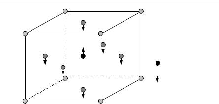
Barium, Ba2+

Titanium, Ti4+

Oxygen, O2–

Fig. 9.4. Unit cell of barium titanate. The displacive transition is indicated by the direction of the arrows

In a little more detail, displacive ferroelectrics involve transitions associated with the displacement of a whole sublattice. How this could arises is discussed in Sect. 9.3.3 where we talk about the soft mode model. The soft mode theory, introduced in 1960, has turned out to be a unifying principle in ferroelectricity (see Lines and Glass [9.12]). Order–disorder ferroelectrics have transitions associated with the ordering of ions. We have mentioned in this regard KH2PO4 as a crystal with hydrogen bonds in which the motion of protons is important. Ferroelectrics have found application as memories, their high dielectric constant is exploited in making capacitors, and ferroelectric cooling is another area of application.

Other examples include ferroelectric cubic perovskite (PZT) PbZr(x)Ti(1–x)O3, Tc = 670 K. The ferroelectric BaMgF4 (BMF) does not show a Curie T even up to melting. These are other familiar ferroelectrics as given below.

The central problem of ferroelectricity is to be able to describe the onset of spontaneous polarization. Spontaneous polarization is said to exist if, in the absence of an electric field, the free energy is minimum for a finite value of the polarization. There may be some ordering involved in a ferroelectric transition, as in a ferromagnetic transition, but the two differ by the fact that the ferroelectric transition in a solid always involves the creation of dipoles.

Just as for ferromagnets, a ferroelectric crystal undergoes a phase transition from the paraelectric phase to the ferroelectric phase, typically, as the temperature is lowered. The transition can be either first order (with a latent heat, i.e. BaTiO3) or second order (without latent heat, i.e. LiTaO3). Just as for ferromagnets, the ferroelectric will typically split into domains of varying size and orientation of polarization. The domain structure forms to reduce the energy. Ferroelectrics show hysteresis effects just like ferromagnets. Although we will not discuss it here, it is also possible to have antiferroelectrics that one can think of as arising from antiparallel orientation of neighboring unit cells. A simple model of spontaneous polarization is obtained if we use the Clausius–Mossotti equation and assume (unrealistically for solids) that polarization arises from orientation effects. This is discussed briefly in a later section.

Соседние файлы в предмете Химия