12.7 Classical and Quantum Hall Effect (A) 629
Fig. 12.14. Schematic diagram of classical Hall effect
Define na as the number of electrons per unit area (projected into the (x,y)-plane) so the Hall voltage can be written
VH = I x B . nae
The Hall conductance 1/Rxy is
1 |
= |
|
I x |
= |
nae |
. |
R |
|
V |
|
xy |
|
|
B |
|
|
|
H |
|
|
|
Longitudinally over a length L, the voltage change is
VL = Ex L = |
J x L |
= |
I x L |
, |
|
|
|
σ0 |
twσ0 |
which we find to be independent of B. This is the usual Drude result. However, this result is based on the assumption that all electrons are moving with the same velocity. If we allow the electrons to have a distribution of velocities by doing a proper Boltzmann equation calculation, we find there is a magnetoresistance effect. The result is (Blakemore [12.3]).
σ = |
|
σ0 |
|
|
|
|
|
|
|
|
. |
(12.30) |
1+ (σ |
R )2 |
|
J × B |
|
2 |
|
|
|
|
0 H |
|
|
|
J |
|
2 |
|
|
|
|
|
|
|
|
|
|
|
|
|
|
|
|
|
|
|
|
|
|
|
|
|
|
|
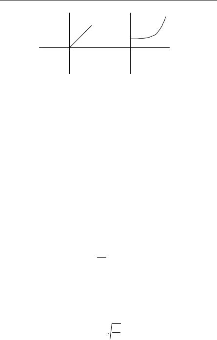
In addition, when band-structure effects are taken into account one finds there also may be a magnetoresistance even when J × B = 0. Classically then we predict behavior for the Hall effect (with Ix = constant) as shown schematically in Fig. 12.15.
630 12 Current Topics in Solid Condensed–Matter Physics
 VH
VH  VL
VL
 B
B
Fig. 12.15. Schematic diagram of classical Hall effect behavior. See (12.27) for VH and (12.29) for VL
12.7.2The Quantum Mechanics of Electrons in a Magnetic Field: The Landau Gauge (A)
We start by solving the problem of electrons moving in two dimensions (x, y) in a magnetic field in the z direction (see, e.g., [12.41, 12.51, 12.56, 12.59]). The essential ideas of the quantum Hall effect can be made clear by ignoring electron spin, and so we do. The limit to two dimensions is necessary for the quantum Hall effect as we will discuss later. The discussion of Landau diamagnetism (Sect. 3.2.2) may be helpful here as a review of the quantum mechanics of electrons in magnetic fields.
For B = Bk, one choice of A is:
A = − |
1 r × B , |
(12.31) |
|
2 |
|
which is a cylindrically symmetric gauge. Instead, we use the Landau gauge where Ax = −yB, Ay = 0, and Az = 0. This yields a simpler solution for the Hall situation that we consider.
The free-electron Hamiltonian can then be written
H = 21m [ p − qA]2 ,
where q = −e < 0. In two dimensions this becomes (compare Sect. 3.2.2)
|
|
1 |
|
|
|
∂ |
|
2 |
2 ∂2 |
|
H |
= |
|
|
|
|
|
− eyB |
− |
|
|
. |
|
i |
|
∂x |
|
∂y2 |
|
|
2m |
|
|
|
|
|
|
|
|
|
|
|
|
|
|
|
|
|
Introducing the “magnetic length”
lμ =  eB ,
eB ,
12.7 Classical and Quantum Hall Effect (A) 631
we can then write the Schrödinger equation as
|
2 |
|
|
|
|
2 |
|
|
|
|
|
|
|
y |
|
2 |
|
|
|
|
|
∂ |
|
|
∂ |
|
|
|
|
|
|
− |
|
|
|
|
|
|
|
1 |
|
|
|
|
|
= Eψ . |
|
|
|
|
|
|
|
|
|
− |
|
|
|
− |
|
|
|
ψ |
|
2m |
∂y |
2 |
∂x |
2 |
|
|
|
|
|
|
|
i |
|
lμ |
|
|
|
|
|
|
|
|
|
|
|
|
|
|
|
|
|
|
|
|
|
|
|
|
|
|
|
We seek a solution of the form |
|
|
|
|
|
|
|
|
|
|
|
|
|
|
|
|
|
|
|
|
|
|
|
ψ = Aeikxϕ( y) , |
|
|
|
and thus |
|
|
|
|
|
|
|
|
|
|
|
|
|
|
|
|
|
|
|
|
|
|
2 |
|
∂ |
2 |
|
|
|
2 |
|
|
( y −lμ2 k)2 |
|
|
− |
|
|
|
|
|
+ |
|
|
|
|
|
ϕ = Eϕ . |
2m |
∂y2 |
|
2ml |
4 |
|
|
|
|
|
|
|
|
|
|
|
|
|
|
|
|
|
|
|
|
|
|
|
|
|
|
μ |
|
|
|
|
|
|
|
|
Since also |
|
|
|
|
|
|
|
|
|
|
|
|
|
|
|
|
|
|
|
|
|
|
|
|
|
|
|
|
|
|
|
lμ = |
|
|
|
mωc |
, |
|
|
|
|
|
|
|
|
|
|
|
|
|
|
|
|
|
|
|
|
|
|
|
|
and from (12.34) and from the preceding equation for lμ, we have
This may be recognized as a harmonic oscillator equation with the quantized energies
En = |
|
1 |
|
…, |
ωc n + |
2 |
, n = 0,1,2 |
|
|
|
|
and the eigenfunctions are
|
|
mω |
1/ 4 |
1 |
|
y |
|
|
|
|
|
1 |
|
y −lμ2 k |
|
2 |
|
|
ϕ |
|
H |
−l |
|
|
− |
|
|
, (12.37) |
n |
= |
|
c |
|
|
μ |
k exp |
|
|
|
|
|
|
|
|
|
|
π |
2n n! |
|
n |
|
|
|
2 |
|
|
lμ |
|
|
|
|
|
|
lμ |
|
|
|
|
|
|
|
|
|
|
|
|
|
|
|
|
|
|
|
|
|
|
|
|
|
|
|
|
|
|
|
|
where the Hn(x) are the Hermite polynomials |
|
|
|
|
|
|
|
|
|
|
|
|
|
|
H0 (x) =1, |
H1(x) = 2x , |
H2 (x) = 4x2 − 2, |
etc. |
|
|
|
|
For the Hall effect we now solve for the case in which there is also an electric field in the y direction (the Hall field). This adds a potential of
The drift velocity in crossed E and B fields is
V = EB ,
632 12 Current Topics in Solid Condensed–Matter Physics
so by (12.38), the above, and ωc = eB/m
|
|
|
|
|
|
|
U = mωcVy . |
|
|
Thus we can write from (12.38): |
|
|
|
|
|
|
2 |
|
∂ |
2 |
|
1 mω2 |
( y −l2 k)2 |
|
|
|
− |
|
|
|
+ |
+ mω Vy |
ϕ = Eϕ . |
|
|
|
|
|
2m ∂y2 |
2 |
c |
μ |
c |
|
|
|
|
|
|
|
|
|
|
|
|
|
|
Now since V is very small, we can neglect terms involving the square of V. Then if we define the origin so y = y′ − aV, with a = 1/ωc, the Schrödinger equation simplifies to the same form as (12.36):
|
|
|
2 |
|
∂ |
2 |
|
1 mωc2 ( y′ −lμ2 k)2 |
|
|
=[E − mωclμ2 kV ]ϕ . |
|
|
− |
|
|
|
+ |
|
ϕ |
|
|
2m ∂y2 |
|
|
|
|
|
2 |
|
|
|
|
|
|
|
|
|
|
|
|
|
|
|
|
|
|
|
|
|
|
|
|
|
|
|
|
|
|
|
|
|
|
|
|
|
Thus using (12.37) in new notation, |
|
|
|
|
|
|
|
|
|
|
|
|
|
|
|
|
|
|
|
y |
+V /ωc |
|
|
|
|
|
|
1 |
|
|
2 |
|
2 |
|
|
|
|
|
|
|
|
|
|
|
|
|
|
|
|
ϕ |
|
H |
|
|
−l |
|
k exp |
− |
|
y +V /ωc −lμk |
|
|
|
, |
n |
|
|
|
μ |
2 |
|
|
|
|
|
|
n |
|
l |
μ |
|
|
|
|
|
l |
μ |
|
|
|
|
|
|
|
|
|
|
|
|
|
|
|
|
|
|
|
|
|
|
|
|
|
|
|
|
|
|
|
|
|
|
|
|
|
|
|
|
|
|
|
|
|
|
and |
|
|
|
|
|
|
|
|
|
|
|
|
|
|
|
|
|
|
|
|
|
|
|
|
|
|
|
|
|
En = ωc |
|
|
1 |
|
|
|
|
2 |
|
|
|
|
|
|
|
|
|
|
|
|
n + |
|
+ mωclμkV . |
|
|
|
|
|
|
|
|
|
|
|
|
|
|
|
|
|
2 |
|
|
|
|
|
|
|
|
|
|
Now let us discuss some qualitative results related to these states.
12.7.3 Quantum Hall Effect: General Comments (A)
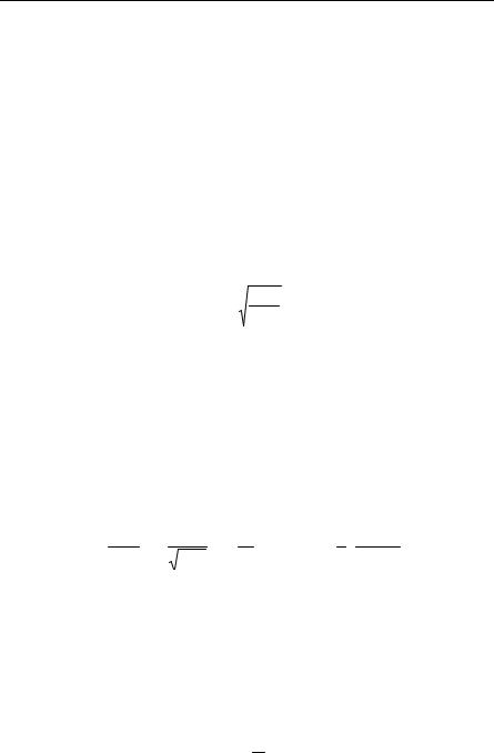
We first present the basic experimental results of the quantum Hall effect and then indicate how it can be explained. We have already described the Hall geometry. The Hall resistance is VH/Ix, where Ix may be held constant. The longitudinal resistance is VL/Ix. One finds plateaus at values of (h/e2)/ν with e2/h being called the quantum of conductance and ν is an integer for the integer quantum Hall effect and a fraction for the fractional quantum Hall effect.
As shown in Fig. 12.16, VL/Ix appears to be zero when the Hall resistance is on a plateau. The figures only schematically illustrate the effect for ν = 2, 1, and 1/3. There are many other plateaus, which we have omitted.
The quantum Hall effect requires two dimensions, low temperatures, electrons, and a large external magnetic field. Two dimensions are necessary so the gaps in between the Landau levels (Eg = ωc) are not obliterated by the continuous energy introduced by motion in the third dimension. (The IQHE involves filled or empty Landau levels. Gaps for the FQHE, which involve partially filled Landau levels, are introduced by electron–electron interactions.) Low temperatures are necessary so as not to wipe out the quantization of levels by thermal-broadening effects.
|
12.7 Classical and Quantum Hall Effect (A) 633 |
|
|
VH/Ix |
VL/Ix |
FQHE |
ν = 1/3 |
3h/e2 |
IQHE |
ν = 1 |
h/e2 |
FQHE |
ν = 2 |
h/2e2 |
Fig. 12.16. Schematic diagram of quantum Hall effect behavior
There are two convenient ways to produce the two dimensional electron systems (2DES). One way is with MOSFETs. In a MOSFET a positive gate voltage can create a 2DES in an inversion region at the Si and SiO2 interface. One can also use GaAs and AlGaAs heterostructures with donor doping in the AlGaAs so the electrons go to the GaAs region that has lower potential. This separates the electrons from the donor impurities and hence the electrons can have high mobility due to low scattering of them.
The IQHE was discovered by Klaus von Klitzing in 1980 and for this he was awarded the Nobel prize in 1985. About two years later, Stormer and Tsui discovered the FQHE and they along with Laughlin (for theory) were awarded the 1998 Nobel prize for this effect.
Qualitatively, the IQHE can be fairly simply explained. As each Landau level is filled there is a gap to the next Landau level. The gap is filled by localized nonconducting states, and as the Fermi level moves through this gap, no change in current is observed. The Landau levels themselves are conducting. For the IQHE the electron–electron interactions effects are really not important, but the disorder that causes the localized states in the gap is crucial.
The fractional quantum Hall effect occurs for partially filled Landau levels and electron–electron interaction effects are crucial. They produce an excitation gap reminiscent of the gap produced in the Mott insulating transition. Potential fluctuations cause localized states and plateau formation.
The Integer Quantum Hall Effect – IQHE–Simple Picture (A)
We give an elementary picture of the IQHE. We start with four results.
a.The Landau degeneracy per spin is eB/h. (This follows because the number of states per unit area in k-space ( A) and in real space is ( A)/(2π)2. Then from (6.29), ( A) = (2π)2(eB/h). Thus, the number of states per unit area in real space is nB ≡ eB/h).
b.The drift velocity perpendicular to E and B field is V = E/B.
c.Flux quanta have the value Φ0 = h/e (see (8.47)).
d.The number of filled Landau levels ν = N/NΦ, where N is the number of electrons and NΦ is the number of flux quanta. This follows from ν = N/(eBLw/h) = N/(Φ/Φ0).
634 12 Current Topics in Solid Condensed–Matter Physics
Then
|
|
|
|
|
|
|
|
|
I x = J xwt = neVwt , |
|
|
|
(12.44) |
where n = the number of electrons per unit volume and |
|
|
|
|
|
|
|
n |
= |
|
|
N |
=ν eB |
(Lw) |
1 |
=ν eB . |
|
|
(12.45) |
|
|
|
wtL |
wtL |
|
|
|
|
|
|
|
|
|
|
|
h |
|
ht |
|
|
|
|
So since V = E/B, |
|
|
|
|
|
|
|
|
|
|
|
|
|
|
|
|
|
|
|
|
|
I x =ν eB e |
E |
wt |
=νe2 Ew |
=νe2 |
VH |
, |
|
(12.46) |
|
|
|
h |
|
|
|
|
|
|
|
|
|
ht |
|
B |
|
h |
|
|
|
|
or |
|
|
|
|
|
|
|
|
|
|
|
|
|
|
|
|
|
|
|
|
I |
|
= |
|
|
1 |
|
= the Hall conductance = |
νe2 |
. |
(12.47) |
V |
|
|
R |
|
|
|
h |
|
|
|
xy |
|
|
|
|
|
|
|
|
|
|
|
H |
|
|
|
|
|
|
|
|
|
|
|
|
|
|
If B changes, as long as the Fermi level stays in the gap, the Landau levels are filled or empty and the current over the voltage remains on a plateau of fixed n. (It can be shown that the total current carried by a full Landau level remains constant even as the number of electrons that fill it varies with the Landau degeneracy.)
Incidentally, when 1/Rxy = νe2/h then 1/Rxx = I/VL → ∞ or Rxx → 0. This is because the electrons in conducting states have no available energy states into which
they can scatter.
Fractional Quantum Hall Effect – FQHE (A)
One needs to think about the FQHE both by thinking about the Laughlin wave functions and by thinking of their physical interpretation. For example, for the ν = 1/3 case with m = 3 (see general comments, next section), the wave function is (see [12.41]):
|
N |
|
1 |
|
|
|
ψ(z1,…, zN ) = ∏ |
(z j − zk )m exp − |
∑Nj =1 |
z j |
|
2 |
|
j<k |
|
4lμ |
|
where zj = xj +iyj locates the jth electron in 2D. Positive and negative excitations at z = z0 are given by (see also [12.59])
|
|
|
|
1 |
|
|
|
|
|
N |
|
N |
|
|
|
ψ + = exp − |
∑Nj =1 |
z j |
2 |
∏(z j − z0 ) ∏(z j − zk )m , |
(12.49) |
|
2 |
|
|
|
|
4lμ |
|
|
|
|
|
j |
|
j<k |
|
|
|
|
1 |
|
|
|
|
2 |
N |
|
∂ |
|
N |
|
|
ψ − = exp |
− |
|
∑N |
z j |
|
∏ |
|
2lμ2 |
− z0 |
∏(z j − zk )m . |
(12.50) |
|
|
|
|
|
|
|
|
2 |
|
j =1 |
|
|
|
j |
|
|
∂z j |
|
|
|
|
|
|
4lμ |
|
|
|
|
|
|
|
|
j<k |
|

12.7 Classical and Quantum Hall Effect (A) 635
For m = 3, these excitations have effective charges of magnitude e/3. The ground state of the FQHE is considered to be like an incompressible fluid as the density is determined by the magnetic field and is fairly rigidly locked. The papers by Laughlin should be consulted for full details.
These wave functions have led to the idea of composite particles (CPs). Rather than considering electrons in 2D in a large magnetic field, it turns out to be possible to consider an equivalent system of electrons plus attached field vortices (see Fig. 16, p. 885 in [12.51]). The attached vortices account for most of the magnetic field and the new particles can be viewed as weakly interacting because the vortices minimize the electron–electron interactions.
General Comments (A)
It turns out that the composite particles may behave as either bosons or fermions according to the number of attached flux quanta. Electrons plus an odd number of surrounding flux quanta are Bose CPs and electrons with an even number of attached quanta are Fermi CPs. The ν = 1/3, m = 3 case involves electrons with three attached quanta and hence these CPs are bosons that can undergo a Bose– Einstein-like condensation, produce an energy gap, and have a FQHE with plateaus. For the ν = 1/2 case, there are two attached quanta, the systems behaves as a collection of fermions, there is no Bose–Einstein condensation and no FQHE.
In general, when the magnetic field increases, electrons can “absorb” some field and become “anyons.” These can be shown to obey fractional statistics and seem to be intermediate between fermions and bosons. This topic takes us too far afield and references should be consulted.2
There are different ways to construct CPs to describe the same physical situation, but normally one tries to use the simplest. Also, there are still problems connected with the understanding of some values of ν. A complete description would take us further than we intend to go, but the chapter references listed at the end of this book can be a good starting point for further investigation.
The quantum Hall effects are very rich in physical effects. So far, they are not so rich in applications. However, the experiments do determine e2/h to three parts in ten million or better, and hence they provide an excellent resistance standard. Also, since the speed of light is a defined quantity, the QHE also determines the fine structure constant e2/ c to high accuracy. It is interesting that the quantum Hall effect determines e2/h, while we found earlier that e/h could be determined by the Josephson effect. Thus the two can be used to determine both e and h individually.
636 12 Current Topics in Solid Condensed–Matter Physics
12.8Carbon – Nanotubes and Fullerene Nanotechnology (EE)
Carbon is very versatile and important both to living tissues and to inanimate materials. Carbon of course forms diamond and graphite. In recent years the ability of carbon to aggregate into fullerenes and nanotubes has been much discussed.
Fullerenes are stable, cage-like molecules of carbon with often a nearly spherical appearance. A C60 molecule is also called a Buckyball. Both are named after Buckminster Fuller because of their resemblance to the geodesic domes he designed. Buckyballs were discovered in 1985 as a byproduct of laser-vaporized graphite. Some of the fullerides (salts such as K-C60) can be superconductors (see, e.g., Hebard [12.25]).
Carbon nanotubes are one or more cylindrical and seamless shells of graphitic sheets. Their ends are capped by half of a fullerene molecule. They were discovered in 1993 by Sumio Iijima and mass produced in 1995 by Rick Smalley. For more details see, e.g., Dresselhaus et al [12.17]. While carbon nanotubes are now easy to produce, they are not easy to produce in a controlled fashion.
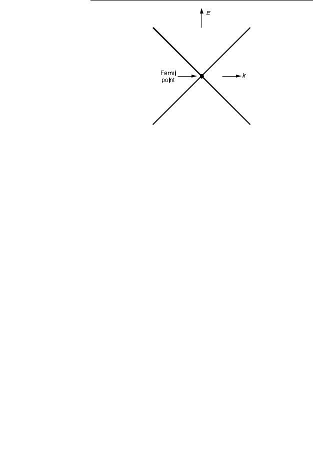
To form them, start with a single sheet of graphite called graphene whose band structure leads to a semimetal (where the conduction band edge is very close to the valence band edge). A picture of the dispersion relations show a twodimensional E vs. k relationship where two cones touch at their tips with the same conic axis and in an end-to-end fashion. See Fig. 12.17. Where the cones touch is the Fermi energy, or as it is called, the Fermi point.
Nanotubes can be semiconductors or metals. It depends on the boundary conditions on the wave function as determined by how the sheet is rolled up. Both the circumference and twist are important. This, in turn, affects whether a bandgap is introduced where the Fermi point in graphene was. The semiconducting bandgap can be varied by the circumference. Multiwalled nanotubes are more complex.
Semiconductor nanotubes can be made to act as transistors by using a gate voltage. A negative bias (to the gate) induces holes and makes them conduct. Positive bias makes the conductance shut off. They have even been made to act as simple logic devices. See McEven PL, “Single-Wall Carbon Nanotubes,” Physics World, pp. 32-36 (June 2000). One interesting feature about nanotubes is that they provide a way around the fundamental size limits of Si devices. This is because they can be made very small and are not plagued with surface states (they have no surface formed by termination of a 3D structure and as cylinders they have no edges).
Carbon nanotubes are a fascinating example of one-dimensional transport in hopefully easy to make structures. They are quantum wires with ballistic electrons
– and they show many interesting quantum effects.
An additional feature of interest is that carbon nanotubes show significant mechanical strength. Their strength arises from the carbon bond.3
3Carbon is becoming an increasingly interesting material with the suggestion that under certain circumstances it can even be magnetic. See Coey M and Sanvito S, Physics World, Nov 2004, p33ff.
12.9 Amorphous Semiconductors and the Mobility Edge (EE) 637
Fig. 12.17. Dispersion relation for graphene
12.9Amorphous Semiconductors and the Mobility Edge (EE)
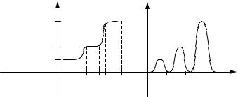
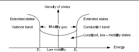
By amorphous, we will mean noncrystalline. Here, rather than an energy gap one has a mobility gap separating localized and nonlocalized states. The localization of electron states is an important concept. The electron–electron interaction itself may give rise to localization as shown by Mott [12.48], as we have discussed earlier in the book. In effect, the electron–electron interaction can split the originally partially filled band into a filled band and an empty band separated by a bandgap. We are more interested here in the Anderson localization transition caused by random local field fluctuations due to disorder. In amorphous semiconductors, this can lead to “mobility edges” rather than band edges (see Fig. 12.18).
The dc conductivity of an amorphous semiconductor is of the form
|
|
|
|
E |
(12.51) |
|
σ =σ0 exp − |
kT |
, |
|
|
|
|
|
|
for charge transport by extended state carriers, where |
E is of the order of the |
|
mobility gap and σ0 is a conductor. For hopping of localized carriers |
|
|
T |
1/ 4 |
|
|
σ =σ0 exp − |
|
0 |
|
, |
(12.52) |
|
T |
|
|
|
|
|
where σ0 and T0 are constants. Memory and switching devices have been made with amorphous chalcogenide semiconductors. The meaning of (12.52) is amplified in the next section.
638 12 Current Topics in Solid Condensed–Matter Physics
Fig. 12.18. Area of mobility between valence and conduction bands
12.9.1 Hopping Conductivity (EE)
So far, we have discussed band conductivity. Here electrons move along at constant energy, in the steady state the energy they gain from the field is dissipated by collisions. One can even have band conductivity in impurity bands when the impurity wave functions overlap sufficiently to form a band. One usually thinks of impurity states as being localized, and for localized states there is no dc conductivity at absolute zero. However, at nonzero temperatures, an electron in a localized state may make a transition to an empty localized state, getting any necessary energy from a phonon, for example. We say the electron hops from state to state. In general, then, an electron hop is a transition of the electron involving both its position and energy.
The topic of hopping conductivity is very complicated and a thorough treatment would take us too far afield. The books by Shoklovskii and Efros [12.55], and Mott [12.48], together with copious references cited therein, can be consulted. In what is given below, we are primarily concerned with hopping conductivity in lightly doped semiconductors.
Suppose the electron jumps to a state a distance R. We assume very low temperatures with the relevant states localized near the Fermi energy. We assume states just below the Fermi energy hop to states just above gaining the energy Ea (from a phonon). Letting N(E) be the number of states per unit volume, we estimate:
|
1 |
≈ |
4 |
πR3N (EF ) , |
(12.53) |
|
Ea |
3 |
|
|
|
|
thus we estimate (see Mott [12.48]) the hopping probability and hence the conductivity is proportional to
exp(−2αR − Ea / kT ) , |
(12.54) |
where α is a constant denoting the rate of exponential decrease of the wave function of the localized state exp(–αr).