8.2 The London and Ginzburg–Landau Equations (B) 467
where |
|
|
|
|
|
|
|
|
|
|
|
|
|
|
|
|
|
|
|
|
|
|
|
|
|
|
|
|
|
λ |
L0 |
|
|
= |
m c2 |
|
. |
|
|
(8.12) |
|
|
|
|
|
|
|
|
|
|
|
|
|
4πn q2 |
|
|
|
|
|
|
|
|
|
|
|
|
|
|
|
|
|
|
|
|
|
|
S |
|
|
|
|
|
|
|
8.2.1 The Coherence Length (B) |
|
|
|
|
|
|
|
|
|
|
|
|
Consider the Ginzburg–Landau |
|
|
equation |
|
in |
the |
|
absence of |
magnetic fields |
(A = 0). Then, in one dimension from (8.3), we have |
|
|
|
|
2 |
|
|
d |
2 |
|
|
|
|
|
|
|
|
|
2 |
|
|
|
|
|
|
|
|
|
|
|
|
|
|
|
|
|
|
|
|
|
|
|
|
|
|
|
|
− |
|
|
|
|
|
|
|
|
|
|
|
|
+α + β |
ψ |
|
ψ = 0 . |
(8.13) |
|
|
|
2m |
|
dx |
2 |
|
|
|
|
|
|
|
|
|
|
|
|
|
|
|
|
|
|
|
|
|
|
|
|
|
|
|
|
|
|
|
|
|
|
|
|
|
|
|
|
|
|
|
|
|
|
|
|
We define |
|
|
|
|
|
|
|
|
|
|
|
|
|
|
|
|
|
|
|
|
|
|
|
|
|
|
f |
= ψ |
|
|
|
where |
ψ0 |
= |
|
− |
α . |
(8.14) |
|
|
|
ψ0 |
|
|
|
|
|
|
|
|
|
|
|
|
|
|
|
|
|
|
β |
|
Then |
|
|
|
|
|
|
|
|
|
|
|
|
|
|
|
|
|
|
|
|
|
|
|
|
|
|
|
|
− |
2 |
|
|
|
d |
2 |
|
|
|
|
|
|
|
2 |
|
|
|
|
|
|
|
|
|
|
|
|
|
|
|
|
|
+1 − |
|
f |
|
|
f |
= 0 . |
(8.15) |
|
|
|
|
|
|
|
|
|
|
2 |
|
|
|
|
|
|
|
|
|
|
|
|
|
|
|
|
|
|
|
|
|
|
|
|
|
|
|
2m |
α dx |
|
|
|
|
|
|
|
|
|
|
|
|
|
|
When f has no gradients | f | = 1, which would correspond to being well inside the superconductor. We assume a boundary at x = 0 between a normal and a superconductor so f = 1, ψ → ψ0 as x → ∞.
Defining
ξ2 (T ) = 2−m 2α and letting f = 1 + g, where g is small, then
ξ 2 (T ) d2g +1+ g − (1+ g)(1+ g)2 = 0 . dx2
Keeping only first order in g since it is small,
ξ2 (T ) d2 g − 2g 0 dx2
g(x) exp[− 2x /ξ(T )] .
(8.16)
(8.17)
(8.18)
(8.19)
Thus, the wave function attains its characteristic value of ψ0 in a distance ξ(T). ξ(T) is called the coherence length. The coherence length measures the “range” or
468 |
8 Superconductivity |
|
|
|
FS – FN |
FS – FN |
|
|
α > 0 |
|
α < 0 |
|
ψ |
ψ0 |
ψ |
|
|
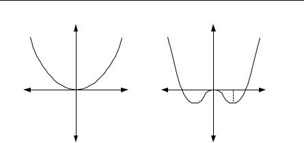
Fig. 8.8. Free energy change at the transition temperature. See (8.20) for how α enters the free energy with no fields or gradients
“size” of Cooper pairs or the distance necessary for the superconducting wave function to change much.
Let us discuss the coherence length further. First, let us review a little about the free energy. The plots for FS − FN are shown in Fig. 8.8. The superconducting transition clearly appears at T = Tc or α = 0. The free energy for no fields or gradients is
F − F |
|
=αψ 2 |
+ |
β |
ψ 4 , |
(8.20) |
|
|
S N |
|
|
2 |
|
|
|
|
|
|
|
|
|
so |
|
|
|
|
|
|
|
|
∂ |
(F − F |
) = 0 |
(8.21) |
|
∂ψ |
|
|
S |
N |
|
|
|
|
gives |
|
|
|
|
|
|
|
|
ψ 2 =ψ02 = − α |
|
(8.22) |
|
|
|
|
|
β |
|
|
at the minimum. Thus at the minimum |
|
|
|
|
|
|
F − F |
= − α2 |
, |
(8.23) |
|
S |
|
N |
|
2β |
|
|
|
|
|
|
|
|
|
which would also be the stabilization energy. From thermodynamics, if F = U − TS, and dU = TdS − MdH, then dF = −MdH at constant T. For perfect diamagnetism,
8.2 The London and Ginzburg–Landau Equations (B) 469
Fig. 8.9. Free energy as a function of field
So,
S 4π
and
FS(H ) − FS(0) = H8π2 .
At H = Hc, the critical field that destroys superconductivity,
FN (Hc ) = FS(Hc ) .
FN is almost independent of H so,
FN (Hc ) = FN (0) . We show the idea schematically in Fig. 8.9. Therefore,
F (0) − F (0) = − |
Hc2 |
= − F |
|
S |
N |
8π |
|
|
|
|
would also be the negative of the stabilization energy, or using (8.23)
Hc2 = α2
8π 2β
H 2
α =  β 4πc .
Notice deep in the superconductor
ψS2 = − αβ = nS = n2 ,
and
λ2 = m c2 . 4π q2nS
(8.26)
(8.27)
(8.28)
(8.29)
(8.30)
(8.31)
(8.32)
(8.33)

|
|
|
|
|
|
So, |
|
|
|
α = −β |
n |
, |
|
(8.34) |
|
2 |
|
|
|
by (8.32) and thus by (8.33) and (8.31) |
|
|
|
α = − |
2e2λ2Hc2 |
. |
(8.35) |
|
|
m c2 |
|
Combining (8.16) and (8.35), an expression for the coherence length can be derived.
We wish to estimate the upper critical field. In Chap. 2 on electrons, we found the allowed energy levels in a constant B field were (in an approximation) free- electron-like parallel to the field and harmonic-oscillator-like in a plane perpendicular to the field. The harmonic energy levels were (dropping * on m)
|
|
1 |
|
|
|
2k 2 |
|
eB |
|
|
|
|
|
|
|
ωc n + |
|
|
= En,kz |
− |
z |
; ωc = |
|
, |
|
2 |
2m |
mc |
|
|
|
|
|
|
|
or
|
|
e |
|
B |
1 |
|
|
2k 2 |
|
|
|
|
|
|
|
|
|
|
|
|
n + |
|
|
= −α − |
z |
, |
(8.36) |
|
|
|
|
|
2 |
2m |
|
|
mc |
|
|
|
|
for the (linearized) Ginzburg–Landau equation (with –α acting as the eigenvalue in (8.3)). The largest value of B for which solutions of the GL equation exists is (n = 0 and letting kz = 0)
B |
≡ H |
c2 |
= − |
2mcα |
. |
(8.37) |
|
|
|
max |
|
|
|
e |
|
|
|
|
|
|
|
|
|
|
The two lengths λ and ξ can be defined as a dimensionless ratio K (the GL parameter). Hc2 can now be described in terms of K and Hc. Using (8.6), (8.16), (8.32), (8.30) and
K = |
λ |
, |
(8.38) |
|
ξ |
|
|
we find |
|
|
|
Hc2 = |
2KHc . |
(8.39) |
If K = λ/ξ > 2−1/2, then Hc2 > Hc. This results in a type II superconductor. The regime of K > 2−1/2 is a regime of negative surface energy.
8.2 The London and Ginzburg–Landau Equations (B) 471
8.2.2 Flux Quantization and Fluxoids (B)
We have for the superconducting current density (by (8.4) with |ψ|2 as spatially constant = n)
Well inside a superconductor J = 0, so
ϕ = qc A .
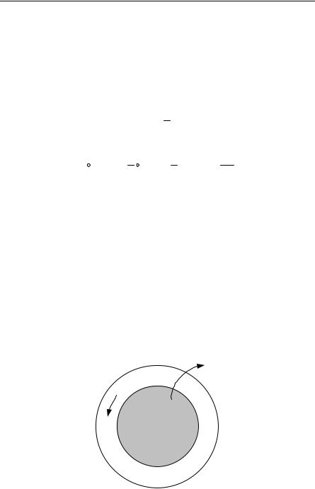
Applying this to Fig. 8.10 and integrating around the loop gives
∫ ϕ dl = qc ∫ A dl = qc ∫S B dS = qcΦ
(2π m) = q Φc ; m = integer
Φ = hcq m ; q = 2e .
This also applies to Fig. 8.11, so
Φ0 = hc2e ≡ the unit of flux of a fluxoid.
(8.40)
(8.41)
(8.42)
(8.43)
(8.44)
(8.45)
In the vortex state of the type II superconductors, the minimum current produces the flux Φ0. In the intermediate state there can be flux tubes threading through the superconductors as shown in Fig. 8.4 and Fig. 8.11. Below, in Fig. 8.12, is a sketch of the penetration depth and coherence length in a superconductor starting with a region of flux penetration. Note λ/ξ < 1 for type I superconductors.
Φ (magnetic flux)
A
J ×
Surface S
loop
Fig. 8.10. Super current in a ring
B
Φ0
Fig. 8.11. Flux tubes in type II superconductors
H  λ
λ
ψ = ψ∞ = ψ0
H
Superconductor
ξ
Fig. 8.12. Decay of H and asymptotic value of superconducting wave function
8.2.3 Order of Magnitude for Coherence Length (B)
For type II superconductors, there is a lower critical field Hc1 for which the flux just begins to penetrate, so
Hc1πλ2 ~ Φ0 |
|
(8.46) |
for a single fluxoid. At the upper critical field, |
|
|
|
H πξ2 ~ Φ |
0 |
, |
(8.47) |
c2 |
0 |
|
|
|
|
|
so that, by (8.44) with m = 1, |
|
|
|
|
|
|
|
ξ02 hc |
1 |
|
1 |
|
(8.48) |
|
|
|
|
2e π Hc2 |
|
for fluxoids packed as closely as possible. ξ0 is the intrinsic coherence length, to be distinguished from the actual coherence length when the superconductor is “dirty” or possessed of appreciable impurities. A better estimate, based on fundamental parameters is1
8.3 Tunneling (B, EE) 473
where vF is the velocity of the Fermi surface and Eg is the energy gap. The coherence length changes in the presence of scattering. If the electron mean free path is l we have
as given by (8.49) for clean superconductors when ξ0 < l and
ξ |
l ξ0 , |
(8.51) |
|
|
ξ/ξ0 |
K > 1 |
K < 1 |
|
II |
I |
|
|
|
λ/ξ0 |
|
|
mfp |
|
|
ξ0 |
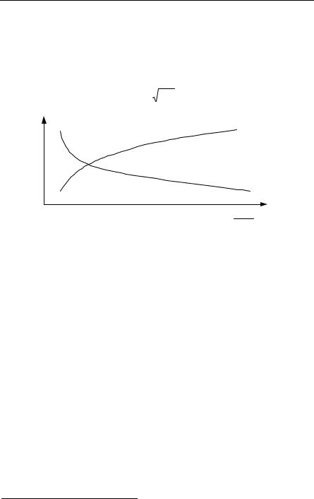
Fig. 8.13. Type I and type II superconductors depending on mfp
for dirty superconductors when l << ξ0.(2) That is, dirty superconductors have decreased ξ and increased K = λ/ξ. The penetration depth can also depend on structure. The idea is schematically shown in Fig. 8.13 where typically the more impure the superconductor the lower the mean free path (mfp) leading to type II behavior.
8.3 Tunneling (B, EE)
8.3.1 Single-Particle or Giaever Tunneling
We anticipate some results of the BCS theory, which we will discuss later. As we will show, when electrons are well separated the electron–lattice interaction can lead to an effective attractive interaction between the electrons. An effective attractive interaction between electrons can cause there to be an energy gap in the single-particle density of states, as we also show later. This energy gap separates the ground state from the excited states and is responsible for most of the unique properties of superconductors.
2 See Saint-James et al [8.27 p. 141]
474 |
8 Superconductivity |
|
|
|
E |
|
E |
|
(1) |
Thin |
(2) |
|
Superconductor |
Normal metal |
|
Insulator |
|
|
(oxide) |
|
|
D(E) |
Eg |
D(E) |
|
|
Fig. 8.14. Diagram of energy gap in a superconductor. D(E) is the density of states
Suppose we form a structure as given in Fig. 8.14. Let T be a tunneling matrix element. For the tunneling current we can write (with an applied voltage V)3
|
I1→2 |
= K′∫ |
∞ |
|
T |
|
2 D1(E) f (E)D2 (E + eV )[1− f (E + eV )]dE |
(8.52) |
|
|
|
|
|
|
|
−∞ |
|
|
|
2 D1(E)D2 (E + eV ) f (E + eV )[1− f (E)]dE |
|
|
I2→1 |
= K′∫ |
∞ |
|
T |
|
(8.53) |
|
|
|
|
|
|
|
−∞ |
|
|
|
|
∞ |
|
|
|
|
|
2 D (E)D (E + eV )[ f (E) − f (E + eV )]dE (8.54) |
I = I |
|
− I |
2→1 |
= K′ |
|
T |
|
|
|
|
1→2 |
|
|
|
|
|
|
∫ |
|
|
|
|
|
|
1 |
2 |
|
|
|
|
|
|
|
|
|
|
|
|
−∞ |
|
|
|
|
|
|
|
2 ∫∞ |
D1S (E) − |
∂f |
eV dE . |
|
|
|
|
|
I K′D2 (0) |
|
T |
|
(8.55) |
|
|
|
|
|
|
|
|
|
|
|
|
|
|
|
|
|
|
|
|
|
|
|
|
|
|
|
|
|
−∞ |
|
|
|
|
|
|
|
|
|
|
|
|
|
|
|
|
|
|
|
|
|
|
∂E |
|
|
4 In the above, K′ is a constant, Di represents density of states, and f is the Fermi function. If we raise the voltage V by eV = , we get the following (see Fig. 8.15) for the net current, and thus, the energy gap can be determined.
3Note this is actually an oversimplified semiconductor-like picture of a complicated many-body effect [8.14 p. 247], but the picture works well for certain aspects and certainly is the simplest way to get a feel for the experiment.
4For the superconducting density of states see Problem 8.2.

8.3 Tunneling (B, EE) 475
Fig. 8.15. Schematic of Giaever (single-particle) tunneling
8.3.2 Josephson Junction Tunneling
Josephson [8.18] predicted that when two superconductors were separated by an insulator there could be tunneling of Cooper pairs from one to the other provided the insulator was thinner than the coherence length, see Fig. 8.16.
The main concept used to discuss the Josephson effects is that of the phase of the paired electrons. We have already considered this idea in our discussion of flux quantization. F. London had the idea of something like a phase associated with superconducting electrons in that he believed that the motions of electrons in superconductors are correlated over large distances. We now associate the idea of spatial correlation of electrons with the idea of the existence of Cooper pairs. Cooper pairs are sets of two electrons that are attracted to one another (in spite of their Coulomb repulsion) because an electron attracts positive ions. As alluded to earlier, the positive ions in a crystal are much more massive and have, in general, less freedom of movement than the conduction electrons. This means that when an electron has attracted a positive ion to a displaced position, we can imagine the electron as moving out of the area while the positive ion remains displaced for a time. In the region of the crystal where the positive ion(s) is (are) displaced, the crystal has a more positive charge than usual and so this region can attract another electron. We could generalize this argument to consider that the displaced positive ion would be undergoing some sort of motion but still an electron with suitable phase could be attracted to the region of the displaced positive ion. Anyway, the argument seems to make it plausible that there can be an effective attractive interaction between electrons due to the presence of the positive ion lattice. The rather qualitative picture that we have given seems to be the physical content of the statement “Cooper pairs of electrons are formed because of the virtual exchange
Superconductor Oxide Superconductor
Fig. 8.16. Schematic of Josephson junction
of phonons between the electrons.” We also see that only lattices in which the electron–lattice vibration coupling is strong will be good superconductors. Thus, we are led to an understanding of the almost paradoxical fact that good conductors of electricity (with low resistance and hence low electron–phonon coupling) often make poor superconductors. We give details including the role of spin later.
Due to the nature of the attractive mechanism between electrons in a Cooper pair, we should not be surprised that the binding of the electrons is very weak. This means that we have to think of the Cooper pairs as being very large (of the order of many, many lattice spacings) and hence the Cooper pairs overlap with each other a great deal in the solid. As we will see, further analysis of the pairs shows that the electrons in pairs have equal and opposite momentum (in the ground state) and equal and opposite spin. However, the Cooper pairs can accept momentum in such a way that they are still “stable” systems, but so that their center of mass moves. When this happens, the motion of the pairs is influenced by the fact that they are so large many of them must overlap. The Cooper pairs are composed of electrons, and the way electronic wave functions can overlap is limited by the Pauli principle. We now know that overlapping together with the constraint of the Pauli principle causes all Cooper pairs to have the same phase and the same momentum (i.e. the momentum of the center of mass of the Cooper pairs). The pairs are like bosons, in a sense, and condense into a lowest quantum state producing a wave function with phase.
Returning to the coupling of superconductors through an oxide layer, we write a sort of time-dependent “Ginzburg–Landau equations,” that allow for coupling,5
i |
|
∂ψ1 |
= H ψ |
1 |
+ |
Uψ |
2 |
, |
(8.56) |
|
|
|
|
∂t |
1 |
|
|
|
|
|
|
|
|
|
|
|
|
|
|
|
|
|
|
|
i |
∂ψ2 |
= H ψ |
2 |
+ |
Uψ |
1 |
. |
(8.57) |
|
|
|
∂t |
2 |
|
|
|
|
|
|
|
|
|
|
|
|
|
|
|
|
|
|
|
If no voltage or magnetic field is applied, we can assume H1 = H2 = 0. Then
|
i |
∂ψ1 |
= |
Uψ2 , |
(8.58) |
|
∂t |
|
|
|
|
|
|
|
i |
∂ψ2 |
|
= |
Uψ1 . |
(8.59) |
|
∂t |
|
|
|
|
|
|
|
5See, e.g., Feynman et al [8.13], and Josephson [8.18], this was Josephson’s Nobel Prize address. See also Dalven [8.11] and Kittel [23 Chap. 12].