Добавил:

Mendeleev Опубликованный материал нарушает ваши авторские права? Сообщите нам.

Вуз:

Российский химико-технологический университет им. Д.И. Менделеева

Предмет:

Химия

Файл:

Patterson, Bailey - Solid State Physics Introduction to theory

.pdf

Скачиваний:

1117

Добавлен:

08.01.2014

Размер:

7.07 Mб

Скачать

☆

<<< < Предыдущая 44 45 46 47 48 49 50 51 52 53 54 5556 / 7356 57 58 59 60 61 62 63 64 65 66 67 68 > Следующая >>>

538 9 Dielectrics and Ferroelectrics

We write out (9.147) to first order for two interesting cases:

Ck +q (t) = λCk(1+) q (t)

	1	(9.150)
=		f0 (k) exp(−i(Ek − Ek +q )t / )V exp(iωt) exp(αt) ,
i

Ck −q (t) = λCk(1−) q (t)

1			f0 (k) exp(−i(Ek − Ek −q )t /						(9.151)
=			f0 (k) exp(−i(Ek − Ek −q )t /				)V exp(−iωt) exp(αt) .
i
Integrating, we find, since Ck±q(∞) = 0
Ck +q (t) =	f0		(k)	exp(−i(Ek − Ek +q )t /		)V exp(iωt) exp(αt)		,	(9.152)
Ck +q (t) =	f0		(k)	Ek − Ek +q		−	ω + i α	,	(9.152)
				Ek − Ek +q		−	ω + i α
Ck −q (t) =	f0	(k)		exp(−i(Ek − Ek −q )t /		)V exp(−iωt) exp(αt)		.	(9.153)
Ck −q (t) =	f0	(k)		Ek − Ek −q		+	ω + i α	.	(9.153)
				Ek − Ek −q		+	ω + i α
We write (9.142) as
	ψ (k) = ∑k′Ck′(t) exp(−iEk′t /						)ψk′ ,		(9.154)
where
				ψk′(r) =	1 eik′ r	,			(9.155)
					Ω

and Ω is the volume. We put a superscript on ψ because we assume we start in the state k. More specifically, (9.153) can be written as

ψ (k) = exp(−iEkt / ) f0 (k)ψk	(9.156)
+ Ck +q (t) exp(−iEk +qt / )ψk +q + Ck −q (t) exp(−iEk −qt / )ψk −q.

Any charge density in jellium is an induced charge density (in equilibrium, jellium is uniform and has a net density of zero). Thus,

ρind

= eN

− e∑

ψ (k)

2 .

(9.157)

Now, note

ψ (k)

2 =

and

∑all k f0 (k) = N ,

(9.158)

9.5 Free-Electron Screening 539

so putting (9.155) into (9.156) and retaining no terms beyond first order,

ind

V exp( iq r )exp( iωt )exp(αt )

∑k

−

( k ) 1+

Ek − Ek+q −

ω +i α

(9.159)

V exp( −iq r )exp(

−iωt )exp(αt )

+ c.c. ,

Ek − Ek+q +

ω +i α

(k) − f

(k + q)]V exp(iq r) exp(iωt) exp(αt)

ρind

∑

[ f

= −

+ c.c.

.(9.160)

Ek − Ek +q − ω + i α

Using

V (q,ω) = −eϕ(q,ω) ,

(9.161)

and identifying ρind(q, ω) as the coefficient of exp(iq r)exp(iωt), we have

	e	2			f		(k) − f
ρind (q,ω) = −	e		∑		f	0	(k) − f	0	(k − q)
						0		0		ϕ(q,ω) .
	Ω									ϕ(q,ω) .
	Ω			k Ek −q − Ek −					ω + i α

By (9.134) we find g(q, ω) and by (9.137), we thus find

ε(q,ω) =1+	e2	∑k	f0 (k) − f0 (k − q)
				.
	εΩq2		Ek −q − Ek − ω + i α

(9.162)

(9.163)

Finally, a few notes are provided on notation. We can redefine the Fourier components so as to change the sign of q. For example, we can say

ϕ(r) =	1	∫ exp(−iq r)ϕ(q)dq .
ϕ(r) =		∫ exp(−iq r)ϕ(q)dq .
(2π)2
Then defining
	vq	=	e2	,
	vq	=	ε Ω q2	,
			ε Ω q2

gives ε(q, ω) in the form given in many textbooks:

ε(q,ω) =1	− vq ∑k	f0 (k + q) − f0 (k)		.
		Ek +q − Ek − ω + i	α

(9.164)

(9.165)

(9.166)

540 9 Dielectrics and Ferroelectrics

The limit as α → 0 is tacitly implied in (9.166). In the limit as q becomes small, (9.165) gives, as we will show below, the Thomas–Fermi approximation (when ω = 0). Two notable effects follow from (9.165), but they are not included in the small q limit. An expression for ε(q,0) at large q is readily obtained for our freeelectron case. The result for ω = 0 is

	1	+	1− x2	ln	1+ x			(9.167)

ε(q,ω) =1+ (constant)D(EF )	2		4x		1	− x	,

where D(EF) is the density of states at the Fermi energy and x = q/2kF with kF being the wave vector at the Fermi energy. This expression has a singularity at q = 2kF, which causes the screening of a charged impurity to have a weakly decaying oscillating term (beyond the Fermi–Thomas potential). This is the origin of Friedel oscillations. The Friedel oscillations damp out with distance due to electron scattering. At finite temperature, the singularity disappears causing the Friedel oscillation to damp out.

Further, since ion–ion interactions are screening by ε(q), the singularity at q = 2kF is reflected in the phonon spectrum. Kinks in the phonon spectrum due to the singularity in ε(q) are called Kohn anomalies.

Finally, we look at (9.165) for small q, ω = 0 and α = 0. We find

ε(q,ω) =1−	e2		∑k	∂f0 / ∂k
	ε Ω q2			∂Ek / ∂k			kS2		(9.168)
	e2				∂f
=1−		∑k D(E)				dE =1+		.
					∂E
	εq2						q2

and hence comparing to previous work, we get exactly the Thomas–Fermi approximation.

Problems

9.1Show that E′0 = E0 + P/ε0, where E0 is the electric field between the plates before the slab is inserted (9.19).

9.2Show that E1 = −P/ε0 (see Fig. 9.2).

9.3Show that E2 = P/3ε0 (9.23).

9.4Show for cubic crystals that E3 = 0 (chapter notation is used).

9.5If we have N permanent free dipoles p per unit volume in an electric field E,

find an expression for the polarization. At high temperatures show that the polarizability (per molecule) is α = p2/3kT. What magnetic situation is this analogous to?

Problems 541

9.6 Use (9.30) and (9.48) to show (9.49)

ε		=1	+		Np2		.
ε	0			3kε	0	(T −T )

						c

Find Tc. How likely is this to apply to any real material?

9.7Use the trial wave function ψ = ψ100 (1 + pz) (where p is the variational parameter) for a hydrogen atom (in an external electric field in the z direction)

to show that we obtain for the polarizability 16πε0a03. (ψ100 is the groundstate wave function of the unperturbed hydrogen atom, a0 is the radius of the

first Bohr orbit of the hydrogen atom, and the exact polarizability is 18πε0a03.)

9.8 (a) Given the Gibbs free energy

G = G	+ 1 β(T −T )P2		+ 1 γP4	+ 1 δP6 ;
0	2	0	4	6
β,δ > 0 , γ < 0		(first order),

derive an expression for Tc in terms of Psc where G(Psc) = G0 and E = 0.

(b) Put the expression for Tc in terms without Psc. That is, fill in the details of Sect. 9.3.1.

10 Optical Properties of Solids

10.1 Introduction (B)

The organization of a solid-state course may vary towards its middle or end. Logical beginnings are fairly easy. One defines the solid-state universe, and this is done with a Section on crystal structures and how they are determined. Then one introduces the main players, and so there are sections on lattice vibrations, phonons, band structure, and electrons. Following this, one can present topics based on the interaction of electrons and phonons and hence discuss, for example, transport. After that come specific materials (semiconductors, magnetic materials, metals, and superconductors) and properties (dielectric, optic, defect, surface, etc). The problem is that some of these categories overlap so that a clean separation is not possible. Optical properties, in particular, seem to spread into many areas, so a well-focused segment on the optical properties of solids can be somewhat tricky to put together.1

By optical properties of solids, we mean those properties that relate to the interaction of solids with electromagnetic radiation whose wavelength is in the infrared to the ultraviolet. There are several aspects to optical properties of solids and looking at the subject in full generality can often lead to complexity, whereas treating each part as a separate case often leads to confusion. We will try to keep to a middle ground between these, by emphasizing only one topic (absorption) but treating it in some detail. Although we will concentrate on absorption, we will mention other optical phenomena including emission, reflection, scattering, and photoemission of electrons.

There are several processes involved in absorption, but the main five seem to be:

(a)Absorption due to electronic transitions between bands that involve wavelengths typically less than ten micrometers;

(b)Absorption by excitons at wavelengths with energies just below the absorption edge due to valence–conduction band transitions (in semiconductors);

(c)Excitation and ionization of impurities that involve wavelengths ranging from about one micrometer to one thousand micrometers;

1 A good treatment is Fox [10.12].

544 10 Optical Properties of Solids

(d)Excitation of lattice vibrations (optical phonons) in polar solids for which the usual wavelengths are ten to fifty micrometers;

(e)Free-carrier absorption for frequencies up to the plasma edge. Free-carrier absorption is particularly important in metals, of course. By gathering data about any optical process, we can gain information about the inner workings of the solid.

10.2 Macroscopic Properties (B)

We start by relating the dielectric properties to optical properties, particularly those involving absorption and reflection. The complex dielectric constant, and the relation of its two components by the Kronig–Kramers relation, is particularly important. The imaginary part relates to the absorption coefficient. We assume the

total charge density ρtotal = 0, j = σE, and μ = μ0 (no internal magnetic effects, all in the usual notation). We assume a wavelength large compared with atomic dimen-

sions but small compared with the dimensions of the sample. We start with Maxwell’s equations and the constitutive relations in SI in the usual notation:

E = 0 × E = −μ0 ∂∂Ht = − ∂∂ Bt

B = 0 × H = j + ∂∂Dt

D = ε0 E+ P = ε E

B = μ0 (H + M) = μ H .

One then finds

2 E = μ σ	∂E	+ μ		∂ 2	(εE) .
	∂t		0 ∂t2
0

We look for solutions for each Fourier component

E(k,ω) = E0 exp[i(k r −ωt)] ,

and keep in mind that ε should be written ε(k, ω). Substituting, one finds k 2 = μ0 (εω2 + iσω) .

Or, since c = 1/(μ0ε0)1/2,

	ω	ε			σ	1/ 2
k =				+ i		.
	c	ε
			0		ε ω
					0

For an insulator, σ = 0 so,
k =	ω	=	ωn	=	ω	ε .
	v		c		c	ε0

(10.1)

(10.2)

(10.3)

(10.4)

(10.5)

(10.6)

10.2 Macroscopic Properties (B)	545

where n is the index of refraction. It is then natural to define a complex dielectric constant εc and a complex index of refraction nc so,

k =	ω n ,	(10.7)
	c c

where

n = ε		+ i	σ = n + in .
c	ε0		ε0ω	i
	ε0		ε0ω
Letting
εc = εr + iεi =			ε(k,ω) + i	σ	,
εc = εr + iεi =			ε(k,ω) + i	ε0ω	,
			ε0	ε0ω

squaring both sides and equating real and imaginary parts, we find

εr (k,ω) = n2 − ni2 ,

and

εi (k,ω) = 2nni .

Now, assuming the wave propagates in the z direction, if we substitute

k = ωc (n + ini ) ,

we have

(10.8)

(10.9)

(10.10)

(10.11)

(10.12)

	nz			−	ω		(10.13)
E = E0 exp iω		c	−t exp		c	ni z .

So, since energy in the wave is proportional to |E|2, we have that the absorption coefficient is given by

α =	2niω	.	(10.14)

	c

Another readily measured quantity can be related to n and ni. If we apply appropriate boundary conditions to a solid surface, we can show as noted below that the reflection coefficient for normal incidence is given by

	(n −1)	2 + n2
R =		i	.	(10.15)
	(n +1)
		2 + n2
		i

This relation follows directly from the Maxwell relations. From Faraday’s law, we can show that the tangential component of E is continuous, and from Ampere’s Law we can show the tangential component of H is continuous. Further manipulation

546 10 Optical Properties of Solids

leads to the desired relation. Let us work this out. For normal incidence from the vacuum on a surface at z = 0, the incident and reflected waves can be written as


	z			z
Ei+r = E1 exp iω		−t	+ E2 exp −iω		+
Ei+r = E1 exp iω		−t	+ E2 exp −iω		+
	c			c

and the refracted wave is given by

		z
Erf	= E0 exp iω nc		−t	,
Erf	= E0 exp iω nc	c	−t	,
		c

where nc is the complex index of refraction. Since

× E + ∂∂Bt = 0 , we can use the loop of Fig. 10.1 to write

∫A ( × E) ds + ∫ ∂∂Bt ds = 0 ,

∫C E dr = − ddt ∫ B ds ,

(ET1 − ET2 ) l + O(ε) = − ddt (B 2lε) ,

t ,

(10.16)

(10.17)

(10.18)

(10.19)

(10.20)

(10.21)

where the subscript T means the tangential component of the electric field, and the subscript means perpendicular to the page of the paper. Taking the limit as ε → 0, we obtain

E1		− E2 = 0 ,			(10.22)
	T	T
or the tangential component of E is continuous. In a similar way we can use
× H = j +			∂D		(10.23)
× H = j +			∂t		(10.23)
			∂t
to show that
(HT1 − HT2 ) l + O(ε) = ∫A j ds +	d	(D 2lε) = j (2lε) +		d	(D 2lε) . (10.24)
(HT1 − HT2 ) l + O(ε) = ∫A j ds +	dt	(D 2lε) = j (2lε) +		dt	(D 2lε) . (10.24)
	dt			dt
Again taking the limit as ε → 0, we find
(HT1 − HT2 ) = 0 ,					(10.25)

10.2 Macroscopic Properties (B)	547

	l
ε	A	2
ε

	ε	1
		1

Curve C

Fig. 10.1. Loop used for deriving field boundary conditions (notice this ε is a distance)

or that the tangential component of H is also continuous. Continuity of the tangential component of H requires (using ×E = −∂B/∂t, proper constitutive relations, and (10.16) and (10.17))

nc E0 = E1 − E2 .

(10.26)

Continuity of the tangential component of E requires ((10.16) and (10.17))

E0 = E1 + E2 .

(10.27)

Adding these two equations gives

E =	E0 (nc +1)	.	(10.28)

1	2

Subtracting these equations gives

E2 =	E0 (−nc +1)	.	(10.29)
	2

Thus, the reflection coefficient is given by

1− n

(n −1)

2 + n2

R =

(10.30)

1+ nc

(n +1)

2 + n2

Enough has been said to indicate that the theory of the optical properties of solids is intimately related to the complex index of refraction of solids. The complex dielectric constant equals the square of the complex index of refraction. Thus, the optical properties of solids are intimately related to the study of the dielectric properties of solids, and the measurement of the absorptivity and reflectivity determine n and ni, and hence, εr and εi.

548 10 Optical Properties of Solids

10.2.1 Kronig–Kramers Relations (A)

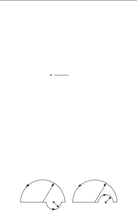
We will give a quantum description of the absorption of radiation, but first it is helpful to derive the Kronig–Kramers equations, which give a relation between the real and imaginary parts of the dielectric constant. Let ε be a complex function of ω that converges in the upper half-plane. We need to define the Cauchy principal value P with a real for the following equations and diagrams:

P∫∞ ε(ω)dω		= 1	∫		ε(ω)dω + ∫		ε(ω)dω	,	(10.31)
−∞	ω − a	2		C′	ω − a	C′′	ω − a

as shown by Fig. 10.2. It is assumed that the integral over the large semicircles is zero. From complex variables, we know that if C encloses a and if f has no singularity in C, then

∫	f (Z)dZ	= 2πi f (a) .
C	Z − a

Using the definition of Cauchy principal value, since we have the integral

	∫ = 0 , P →				1
	∫ = 0 , P →				2		∫ − ∫ .
	C′′				2	C′ C′′
Thus,
P∫	ε(ω)dω	=	1	∫		ε(ω)dω		= iπε(a) ,
	ω − a		2 smallcircle				ω − a
				ρ→0

(10.32)

(10.33)

(10.34)

and we have used that ε(ω) on the big circle is zero (actually, to achieve this we should use that ε(ω) = [εr(ω) − 1] + iεi(ω), which we will put in explicitly at the end). Taking real and imaginary parts we then have,

P∫∞	Re[ε(ω)]dω	= −π Im[ε(a)] ,	(10.35)
−∞	ω − a
and
P∫∞	Im[ε(ω)]dω	= +π Re[ε(a)] .	(10.36)
−∞	ω − a
C′		C″
R → ∞		R → ∞
	ρ → 0	a
	a	a
		ρ → 0
Fig. 10.2. Contours used for Cauchy principal value

<<< < Предыдущая 44 45 46 47 48 49 50 51 52 53 54 5556 / 7356 57 58 59 60 61 62 63 64 65 66 67 68 > Следующая >>>

Соседние файлы в предмете Химия

#
08.01.20149.92 Mб37Martin. Electronic structure - basic theory and practical methods.djvu
#
08.01.201411.89 Mб114Matta, Boyd. The quantum theory of atoms in molecules.pdf
#
08.01.201411.33 Mб58Metal Surface Electron Physics 0080426751.pdf
#
08.01.201412.51 Mб60Molecular Heterogeneous Catalysis, Wiley (2006), 352729662X.pdf
#
08.01.201432.51 Mб48Organic_Chemistry.Oxford_University_Press.Clayden.J,Greeves.N,Warren.S,Wothers.P.2000.pdf
#
08.01.20147.07 Mб1117Patterson, Bailey - Solid State Physics Introduction to theory.pdf
#
08.01.201413.22 Mб69Quantum-Mechanical Prediction of Thermochemical Data.pdf
#
08.01.201412.65 Mб186Reactive Intermediate Chemistry.pdf
#
04.05.201468.94 Mб70Roberts, Caserio - Basic Principles of Organic Chemistry (2nd edition, 1977).pdf
#
08.01.201418.06 Mб29Smith M.B., March J. March's advanced organic chemistry.. reactions, mechanisms, and structure (5ed., Wiley, 2001)(T)(2101s).djvu
#
08.01.201432.12 Mб43Theoretical Organic Chemistry.pdf