Patterson, Bailey - Solid State Physics Introduction to theory

11.6 Edge and Screw Dislocation (MET, MS) 599

where D is, by definition, the diffusion constant. Combining this with the equation of continuity

For solution of this equation, we refer to several well-known treatises as referred to in Borg and Dienes [11.2]. Typically, the diffusion constant is a function of temperature via

where E0 is the activation energy that depends on the process. Interstitial defects moving from one site to an adjacent one typically have much less E0 than say, vacancy motion. Obviously, the thermal variation of defect diffusion rates has wide application.

11.6 Edge and Screw Dislocation (MET, MS)

Any general dislocation is a combination of two basic types: the edge and the screw dislocations. The edge dislocation is perhaps the easiest to describe. If we imagine the pages in a book as being crystal planes, then we can visualize an edge dislocation as a book with half a page (representing a plane of atoms) missing. The edge dislocation is formed by the missing half-plane of atoms. The idea is depicted in Fig. 11.6. The motion of edge dislocations greatly reduces the shear strength of crystals. Originally, the shear strength of a crystal was expected to be much greater than it was actually found to be for real crystals. However, all large crystals have dislocations, and the movement of a dislocation can greatly aid the shearing of a crystal. The idea involves similar reasoning as to why it is easier to move a rug by moving a wrinkle through it rather than moving the whole rug. The force required to move the wrinkle is much less.

Crystals can be strengthened by introducing impurity atoms (or anything else), which will block the motion of dislocations. Dislocations themselves can interfere with each other’s motions and bending crystals can generate dislocations, which then causes work hardening. Long, but thin, crystals called whiskers have been grown with few dislocations (perhaps one screw dislocation to aid growth – see below). Whiskers can have the full theoretical strength of ideal, perfect crystals.

The other type of dislocation is called a screw dislocation. Screw dislocations can be visualized by cutting a book along A (see Fig. 11.7), then moving the upper half of the book a distance of one page and taping the book into a spiral staircase. Another view of the dislocation is shown in Fig. 11.8 where successive atomic

11.7 Thermionic Emission (B) 601

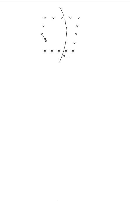
b

Dislocation line

Fig. 11.9. Diagram used for the definition of the Burgers vector b

path is the Burgers vector. For a pure edge dislocation, the Burgers vector is perpendicular to the dislocation line; for a pure screw dislocation, it is parallel. In general, the Burgers vector can make any angle with the dislocation line, which is allowed by crystal symmetry. The book by Cottrell [11.6] is a good source of further details about dislocations. See also deWit [11.9].

11.7 Thermionic Emission (B)

We now discuss two very classic and important properties of the surfaces of metals – in this Section thermionic emission and in the next Section cold-field emission.

So far, we have mentioned the role of Fermi–Dirac statistics in calculating the specific heat, Pauli paramagnetism, and Landau diamagnetism. In this Section we will apply Fermi–Dirac statistics to the emission of electrons by heated metals. It will turn out that the fact that electrons obey Fermi–Dirac statistics is relatively secondary in this situation.

It is also possible to have cold (no heating) emission of electrons. Cold emission of electrons is obtained by applying an electric field and allowing the electrons to tunnel out of the metal. This was one of the earliest triumphs of quantum mechanics in explaining hitherto unexplained phenomena. It will be explained in the next section.5

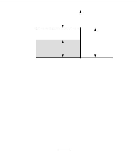
For the purpose of the calculation in this section, the surface of the metal will be pictured as in Fig. 11.10. In Fig. 11.10, EF is the Fermi energy, φ is the work function, and E0 is the barrier height of the potential. The barrier can at least be partially understood by an image charge calculation.

5A comprehensive review of many types of surface phenomena is contained in Gundry and Tompkins [11.14].

11.8 Cold-Field Emission (B) 605

To calculate the current density, which is emitted by the metal when the electric field is applied, it is necessary to have the transmission coefficient for tunneling through the barrier. This transmission coefficient can perhaps be adequately evaluated by use of the WKB approximation. For a high and broad barrier, the WKB approximation gives for the transmission coefficient

x0 is the second classical turning point, and E is, of course, the energy.

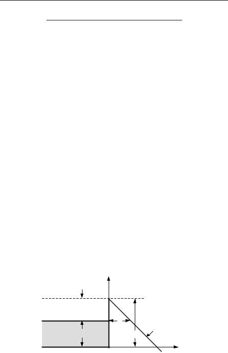
The upper limit of the integral is determined (for an electron of energy E) from

Therefore

∫xx=00 K (x)dx = 32 2m(E0 − E)3 /( eE1)2 .

Since (E0 − EF) = φ, the transmission coefficient for electrons with the Fermi energy is given by

Further analysis shows that the current density for field-emitted electrons is given approximately by J E12T so,

where a and b are different constants for different materials. Equation (11.49), where b is commonly proportional to φ3/2, is often referred to as the Fowler–Nord- heim equation. The ideas of Fowler–Nordheim tunneling are also used for the tunneling of electrons in a metal-oxide-semiconductor (MOS) structure. See also Sarid [11.27].

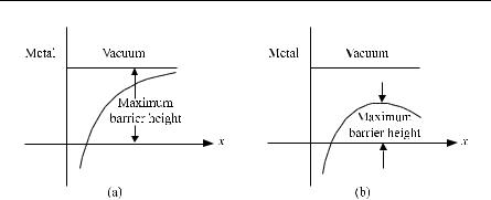
There is another type of electron emission that is present when an electric field is applied. When an electric field is applied, the height of the potential barrier is slightly lowered. Thus more electrons can be classically emitted (without tunneling) by thermionic emission than previously. This additional emission due to the lowering of the barrier is called Schottky emission. If we imagine the barrier is caused by image charge attraction, it is fairly easy to see why the maximum barrier height should decrease with field strength. Simple analysis predicts the barrier lowering to be proportional to the square root of the magnitude of the electric field. The idea is shown in Fig. 11.12. See Problem 11.7.

Problems 607

In a drop tube, there is an enclosure in which, for example, only the molten sample would be dropped. Special aerodynamic design, vacuum, or other means is used to reduce air drag and, hence, obtain real free-fall. For slightly longer times (20 s or so), the KC 135 aircraft can be put into a parabolic path to produce microgravity. Extending this idea, rockets have been used to produce microgravity for periods of about 400 s.

Problems

11.1Give a simple derivation of Ivey’s law. Ivey’s law states that fa2 = constant where f is the frequency of absorption in the F-band and a is the lattice spacing in the colored crystal. Use as a model for the F-center an electron in a box and assume that the absorption is due to a transition between the ground and first excited energy states of the electron in the box.

11.2The F-center absorption energy in NaCl is about 2.7 eV. For a particle in a

box of side aNaCl = 5.63 × 10−10 m, find the excitation energy of an electron from the ground to the first excited state.

11.3A low-angle grain boundary is found with a tilt angle of about 20 s on a (100) surface of Ge. What is the prediction for the linear dislocation density of etch pits predicted?

11.4Find the allowed energies of a hydrogen atom in two dimensions. The answer you should get is [12.54]

En = − (n −R1 )2 ,

2

where n is a nonzero integer. R is the Rydberg constant that can be written as

where K = ε/ε0 with ε the appropriate dielectric constant. Since the Bohr radius is

aB = 4πε0K 2 , me2

one can also write

Note that the result is the same as the three-dimensional hydrogen atom if one replaces n by n − ½.