Patterson, Bailey - Solid State Physics Introduction to theory
.pdf8.3 Tunneling (B, EE) 477
We seek solutions of the form (any complex function can always be written as a product of amplitude ρ and eiφ where φ is the phase)
ψ1 = ρ1 exp(iϕ1) , |
|
(8.60) |
ψ2 = ρ2 exp(iϕ2 ) . |
|
(8.61) |
So, using (8.58) and (8.59) we get |
|
|
iρ1 − ρ1ϕ1 =Uρ2 exp(i |
ϕ) , |
(8.62) |
iρ2 − ρ2ϕ2 =Uρ1 exp(−i |
ϕ) , |
(8.63) |
where |
|
|
ϕ = (ϕ2 −ϕ1) |
|
(8.64) |
is the phase difference between the electrons on the two sides. Separating real and imaginary parts,
ρ1 =Uρ2 sin ϕ , |
(8.65) |
|||||||
ρ1ϕ1 = −Uρ2 cos |
ϕ , |
(8.66) |
||||||
ρ2 = −Uρ1 sin |
ϕ , |
(8.67) |
||||||
ρ2ϕ2 = −Uρ1 cos |
ϕ . |
(8.68) |
||||||
Assume ρ1 ρ2 ρ for identical superconductors, then |
|
|||||||
|
d |
|
(ϕ |
2 |
−ϕ ) = 0 , |
(8.69) |
||
|
|
|||||||
|
dt |
1 |
|
|
||||
|
|
|
|
|
||||
ϕ2 −ϕ1 constant , |
(8.70) |
|||||||
|
|
|
ρ1 −ρ2 . |
|
(8.71) |
|||
The current density J can be written as |
|
|
|
|||||
J |
d |
ρ22 = 2ρ2ρ2 , |
(8.72) |
|||||
dt |
||||||||
|
|
|
|
|
|
|
||
so |
|
|
|
|
||||
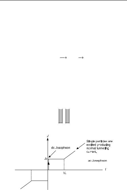
J = J0 sin(ϕ2 −ϕ1) . |
(8.73) |
|||||||
This predicts a dc current with no applied voltage. This is the dc Josephson effect. Another more rigorous derivation of (8.73) is given in Kuper [8.20 p 141]. J0 is the critical current density or the maximum J that can be carried by Cooper pairs.


8.4 SQUID: Superconducting Quantum Interference (EE) 481
where the first term on the right is zero or negligible. So, using Stokes Theorem and B = × A (and choosing a path where J 0)
ϕ1 − |
ϕ2 = |
q |
∫ |
A dl = |
|
q |
|
∫ B dA = qΦ |
. |
(8.92) |
|||||||||||||||||
|
|
c |
|
|
|
|
|
|
|
|
c |
|
|
|
|
|
|
|
|
|
|
|
c |
|
|
||
Defining Φ0 = c/q as per (8.45), we have |
|
|
|
|
|
|
|
|
|
|
|
|
|
|
|
|
|
|
|
|
|
|
|||||
|
|
ϕ − ϕ |
|
|
= |
Φ |
, |
|
|
|
|
|
|
|
|
(8.93) |
|||||||||||
|
|
|
|
|
|
|
|
|
|
|
|
|
|
|
|
||||||||||||
|
|
|
1 |
|
|
2 |
|
|
Φ0 |
|
|
|
|
|
|
|
|
|
|||||||||
so when Φ = 0, and φ1 = |
φ2. We assume the junctions are identical so defining |
||||||||||||||||||||||||||
φ0 = ( φ1 + φ2)/2, then |
|
|
|
|
|
|
|
|
|
|
|
|
|
|
|
|
|
|
|
|
|
|
|
|
|
|
|
|
|
ϕ = ϕ |
0 |
+ |
|
|
Φ |
|
|
|
, |
|
|
|
|
|
|
|
|
(8.94) |
|||||||
|
|
|
|
|
|
|
|
|
|
|
|
|
|
|
|
|
|
||||||||||
|
|
|
1 |
|
|
|
|
2Φ0 |
|
|
|
|
|
|
|
|
|
||||||||||
|
|
|
|
|
|
|
|
|
|
|
|
|
|
|
|
|
|
||||||||||
|
|
ϕ2 |
= ϕ0 − |
|
|
Φ |
|
|
|
|
|
|
|
|
|
|
|
|
|
(8.95) |
|||||||
|
|
|
2Φ0 |
|
|
|
|
|
|
|
|
||||||||||||||||
|
|
|
|
|
|
|
|
|
|
|
|
|
|
|
|
|
|
|
|||||||||
is a solution. By (8.73) |
|
|
|
|
|
|
|
|
|
|
|
|
|
|
|
|
|
|
|
|
|
|
|
|
|
|
|
JT = J1 + J2 = J0 (sin |
|
|
ϕ1 + sin |
ϕ2 ) |
|
|
|
|
|||||||||||||||||||
|
|
ϕ |
+ ϕ |
2 |
|
|
|
|
|
ϕ − |
ϕ |
2 |
(8.96) |
||||||||||||||
= 2J0 sin |
|
1 |
2 |
|
|
|
cos |
1 |
2 |
|
. |
|
|||||||||||||||
|
|
|
|
|
|
|
|
|
|
|
|
|
|
|
|
|
|
|
|
||||||||
So |
|
|
|
|
|
|
|
|
|
|
|
|
|
|
|
|
|
|
|
|
|
|
|
|
|
|
|
|
|
|
|
|
|
|
|
|
|
|
|
|
|
|
|
|
|
|
|
|
|
|
|||||
|
JT = 2J0 sin(ϕ0 ) cos |
|
Φ |
|
, |
|
|
|
(8.97) |
||||||||||||||||||
|
2Φ0 |
|
|
|
|||||||||||||||||||||||
|
|
|
|
|
|
|
|
|
|
|
|
|
|
|
|
|
|
||||||||||
and |
|
|
|
|
|
|
|
|
|
|
|
|
|
|
|
|
|
|
|
|
|
|
|
|
|
|
|
|
|
|
|
|
|
|
|
|
|
|
Φ |
|
|
|
|
|
|
|
|
||||||||
|
|
|
|
|
|
|
|
|
|
|
|
|
|
|
|
||||||||||||
|
JT |
|
= |
2J0 |
|
|
|
|
|
|
|
|
. |
|
|
|
|
(8.98) |
|||||||||
|
|
cos |
|
|
|
|
|
|
|
|
|
|
|
|
|||||||||||||
|
max |
|
|
|
|
|
|
|
2Φ0 |
|
|
|
|
|
|
|
|
||||||||||
The maximum occurs when Φ = 2nπΦ0. Thus, quantum interference can be used to measure small magnetic field changes. The maximum current is a periodic function of Φ and, hence, measures changes in the field. Sensitive magnetometers have been constructed in this way. See the original paper about SQUIDS by Silver and Zimmerman [8.31].
8.4.1 Questions and Answers (B)
Q1. What is the simplest way to understand the dc Josephson effect (a current with no voltage in a super–insulator–super sandwich or SIS)?


8.5 The Theory of Superconductivity (A) |
483 |
|
|
In the above equation, the a are, of course, phonon creation and annihilation operators.
By a second quantization representation of the terms involving electron coordinates (see Appendix G), we can write
∂U (ri ) = ∑ ψk xl,bU (ri ) ψk′ Ck†Ck′ , |
(8.101) |
∂xl,b k,k′ |
|
where the C are electron creation and annihilation operators. The only quantities that we will want to calculate involve matrix elements of the operator Hep. As we have already shown, these matrix elements will vanish unless the selection rule q = k′ − k − Gn is obeyed. Neglecting umklapp processes (assuming Gn = 0 the first major approximation), we can write
H ep = −i∑ ∑ ∑ |
2Nm ω |
q, p |
exp(−iq l) |
|
|
|
|
|
|
|
|
|
|
(8.102) |
||||||||||
l,b q, p k,k′ |
|
|
|
b |
|
|
|
|
|
|
|
|
|
|
|
|
|
|
|
|||||
× ψ |
e* |
|
|
xlb |
U (r ) ψ |
k′ |
δ k′−k (a† |
− a |
−q, p |
)C†C |
k′ |
, |
||||||||||||
|
k q,b, p |
|
|
|
|
i |
|
q |
|
q, p |
|
|
k |
|
|
|||||||||
or |
|
|
|
|
|
|
|
|
|
|
|
|
|
|
|
|
|
|
|
|
|
|
|
|
H ep = −i∑ ∑ ∑ |
2Nm ω |
q, p |
exp(−iq l) |
|
|
|
|
|
|
|
|
|
|
(8.103) |
||||||||||
l,b q, p k,k′ |
|
|
|
b |
|
|
|
|
|
|
|
|
|
|
|
|
|
|
|
|
||||
× ψ |
|
e* |
|
p |
|
xlb |
U (r ) ψ |
k′ |
(a† |
− a |
−q, p |
)C† |
′−q |
C |
k′ |
. |
||||||||
|
k′−q q,b, |
|
|
i |
|
q, p |
|
k |
|
|
|
|||||||||||||
Making the dummy variable changes k′ → k, q → −q, and dropping the sum over p (assuming, for example, that only longitudinal acoustic phonons are effective in the interaction—this is the second major approximation), we find
|
H ep = i ∑ BqCk† |
+qCk (aq − a−†q ) |
(8.104) |
|
k,q |
|
|
where |
|
|
|
Bq = ∑ |
exp(iq l) ψk +q e−*q,b xl,bU (ri ) ψk . |
(8.105) |
|
l,b |
2Nmbωq |
|
|
The only property of Bq that we will use from the above equation is Bq = B−q*. From any reasonable, practical viewpoint, it would be impossible to evaluate the above equation directly and obtain Bq. Thus, Bq will be treated as a parameter to be evaluated from experiment. Note that so far we have not made any approximations that are specifically restricted to superconductivity. The same Hamiltonian could be used in certain electrical-resistivity calculations.

|
8.5 The Theory of Superconductivity |
(A) 485 |
||
|
|
|
|
|
so that |
|
|
|
|
H S |
= H +[H , S] + |
1 |
[[H ,S],S] +…. |
(8.110) |
|
|
2 |
|
|
We can treat the next few terms in a similar way.
The second useful result is obtained by H = H0 + XHep where X is eventually going to be set to one. In addition, we choose S so that
ΧH ep +[H 0 , S] = 0 . |
(8.111) |
We show that in this case HS has no terms of O(X). The result is proved by using (8.110) and substituting H = H0 + XHep. Then
H S = H 0 + ΧH ep + [ H 0 + ΧH ep |
,S ] + |
1 |
[[ H 0 + ΧH ep ,S ],S ] +… |
|
||||||||||||
|
|
|||||||||||||||
|
|
|
|
|
|
|
|
|
|
2 |
|
|
|
|
|
|
= H 0 + X H ep + [ H 0 ,S ] + X [ H ep ,S ] |
|
|
|
(8.112) |
||||||||||||
|
1 |
|
|
X |
|
|
|
|
|
|
|
|
||||
+ |
|
[[ H 0 ,S ],S ] + |
|
[[ H ep ,S ],S ] +…. |
|
|
|
|
||||||||
2 |
2 |
|
|
|
|
|||||||||||
Using (8.111), we obtain |
|
|
|
|
|
|
|
|
||||||||
H S |
= H 0 |
+ X[H ep ,S] + |
X |
[[H ep , S],S] + 1 [[H |
0 , S],S] +… . |
(8.113) |
||||||||||
|
|
|||||||||||||||
|
|
|
2 |
|
|
2 |
|
|
|
|
||||||
Since |
|
|
|
|
|
|
|
|
|
|
|
|
|
|
|
|
|
|
|
ΧH ep +[H 0 , S] = 0 , |
|
|
|
(8.114) |
|||||||||
we have |
|
|
|
|
|
|
|
|
|
|
|
|
|
|
|
|
|
|
|
Χ [H ep , S] = −[[H 0 , S], S] , |
|
|
|
(8.115) |
|||||||||
so that |
|
|
|
|
|
|
|
|
|
|
|
|
|
|
|
|
H S = H 0 + Χ [H ep , S] + |
Χ |
[[H ep , S], S] − |
Χ |
|
[H ep , S] , |
(8.116) |
||||||||||
|
|
|
|
|
|
|
|
|
2 |
|
|
|
2 |
|
|
|
or |
|
|
|
|
|
|
|
|
|
|
|
|
|
|
|
|
|
|
|
H S = H 0 + |
X |
[H ep , S] + O(X 3) . |
|
|
(8.117) |
||||||||
|
|
|
|
|
|
|||||||||||
|
|
|
2 |
|
|
|
|
|
|
|
|
|||||
Since O(S) = X the second term is of order X2, which was to be proved.
The point of this transformation is to push aside terms responsible for ordinary electrical resistivity (third major transformation). In the original Hamiltonian, terms in X contribute to ordinary electrical resistivity in first order.