Environmental Biotechnology - Jordening and Winter

6.4 Hydrodynamic and Liquid Mixing Behavior of the Biogas Tower Reactor 191

· The only parameter that is not known a priori, is the sedimenting mass flow rate Msedi. This value was determined by regression analysis from the experiments performed as shown in Fig. 6.29. It can be clearly seen that the sedimentation capacity of active gassing sludge is much smaller compared to inactive (dead) sludge as used in the laboratory experiment. The sedimentation of active sludge follows Eqs. 29 and 30 where Areactor is the cross-sectional area of the reactor.

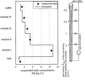
In Figure 6.30 results of experiments and the calculation on the basis of the mathematical model are compared. The agreement between simulated data and measured suspended solid concentration is quite good. The relative deviation between measured and calculated values increases with decreasing concentration of suspended solids. The relative deviation ranges from 10%–15% of the concentrations in the BTR. To investigate the scattering of the measured concentration of suspended solids, 10 samples were taken at one sampling point during a laboratory scale experiment. The detected suspended solid concentrations deviated by up to 8% from the average value. This shows that part of the deviation might be due to sampling errors.

Reinhold and Märkl (1997) also demonstrated that the mathematical model allows for realistic predictions of the dynamic behavior of the system, as was shown by simulating the start-up of a BTR.

Fig. 6.29 Sedimenting mass flow rate between adjacent modules on the laboratory scale and pilot scale as a function of the suspended solid concentration in the upper module.

192 6 Modeling of Biogas Reactors

Fig. 6.30 Concentration of suspended solids as a function of reactor height in the 15 m3 pilot

scale BTR. ·feed = 315 L h–1; total gas production of the reactor 2.3 m3 h–1; gas recirculated 1.8 m3

V

h–1; ÄTOC = 7.3 kg m–3; gas loading Vgas, i of the connecting areas between the modules as indicated.

6.5

Mass Transport from the Liquid Phase to the Gas Phase

As demonstrated in Section 6.3, it is necessary to have quantitative data for the concentrations of the product gases, like CO2, NH3, and H2S in the fermentation broth, to calculate the pH value within the fermentation broth and get information on the kinetics of methane production. To calculate these concentrations it is necessary to have additional information about the transport of these gases from the liquid phase

– where they are produced by the microorganisms – to the gas phase. Basic ideas of this calculation will be discussed with the example of H2S because of its strong influence on biogas production. Polomski (1998) performed experiments on the desorption of H2S from the fermentation liquid broth in laboratory and pilot scale reactors.

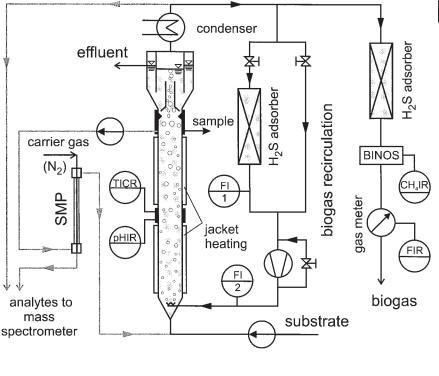
The experimental setup of the laboratory experiment is shown in Figure 6.31. The UASB reactor is supplied with wastewater at the bottom. A part of the generated biogas is withdrawn at the top of the reactor and recycled to the bottom where it is injected by means of a perforated tube. The recycled biogas is either recycled directly or over a H2S adsorber. The H2S concentration in the fermentation liquid and the partial presure of H2S in the gas were measured by means of a silicon membrane probe and the mass spectrometer (see also Section 6.2.1).

6.5 Mass Transport from the Liquid Phase to the Gas Phase 193

Fig. 6.31 Experimental setup of a modified laboratory scale UASB reactor (active volume: 36.5 L) equipped with a bypass membrane probe and a mass spectrometer.

The effect of gas recirculation can be explained with the example of one result of the experiment shown in Figure 6.32. At the ordinate on the left side the H2S partial pressure is denoted; on the right side the H2S concentration in the liquid phase is denoted which is in equilibrium with the partial pressure in the gas according to Eq. 31 and the Henry coefficient HH2S = 2.330 · 10–2 mg L–1 Pa–1 (equal to 6.85 · 10–4 mmol L–1 Pa–1).

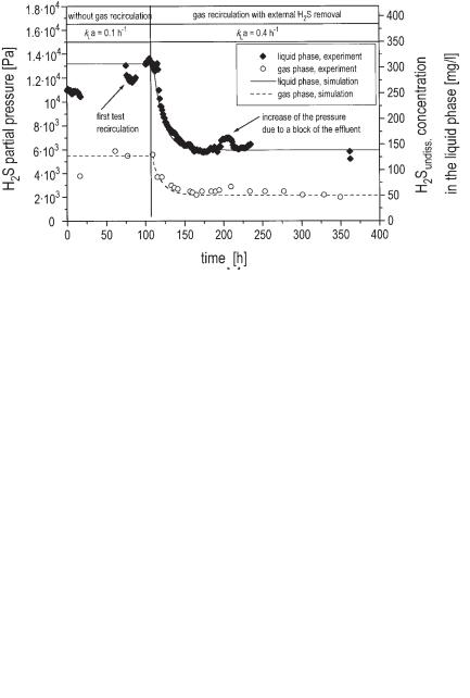
It can be easily seen that in this type of reactor without gas recirculation (first 23 h of the experiment) H2S in the liquid and the gas phases is far from equilibrium. The concentration in the liquid phase is overconcentrated by 75% compared to the gas phase. After recirculating the gas and concurrently producing a larger interfacial area between the liquid and gas phases the overconcentration is diminished to 18%. After starting recirculation of biogas 8 h are required to come from one steady state to the next. In Figure 6.33 the result of a similar experiment is shown. Different from the first one, the recirculated biogas passes a H2S absorber and is eliminated from the system. Although here the sulfate content in the wastewater is extremely

6.5 Mass Transport from the Liquid Phase to the Gas Phase 195

high (5.13 g L–1), the concentration of H2S in the liquid phase can be lowered to 130 mg L–1.

Figures 6.32 and 6.33 also demonstrate that model calculations fit well with the experimental data. The H2S content in the liquid and the gas phases can be calculated by using H2S balances for the different compartments.

6.5.1

Liquid Phase

In Eq. 32 Vreactor is the volume of the liquid in the reactor, cS,tot the concentration of

·

the total sulfur in the liquid according to Eq. 7, V feed is the volumetric feed rate of the reactor and cS,tot,e the concentration of the total sulfur in the reactor feed.

kLa denotes the transport capacity between the liquid phase and the gas phase (a: interfacial area per volume m2 m–3), cH2S is the concentration of the undissociated portion of the H2S in the liquid, and pH2S,bubble the partial pressure of H2S in the bubbles rising in the reactor liquid. HH2S is the Henry coefficient for H2S.

6.5.2

Gas Bubbles

Eq. 33 gives the H2S balance for the gas bubbles in the reactor suspension:

partial pressure of H2S in this flow. V bubble is the volumetric gas production rate of the reactor.

6.5.3

Head Space

Eq. 34 gives the H2S (pH2S) partial pressure in the head space located over the reactor liquid, which is equal to the partial pressure of H2S in the biogas outlet of the reactor:

196 6 Modeling of Biogas Reactors

Vgas is the volume of the head space. Assuming steady state, the partial pressure of H2S in the gas bubbles rising in the biogas suspension pH2S,bubble and the partial pressure of the produced biogas pH2S are equal.

The kLa value in Eqs. 32 and 33 is not known a priori. It can be estimated by a regression analysis, fitting the model calculation to the experimental data. The resulting kLa values are denoted in the Figures 6.32 and 6.33. It can be seen that recirculation of biogas in the experimental reactor of Figure 6.31 increases the kLa value by a factor of 3–4 compared to the situation without gas recirculation.

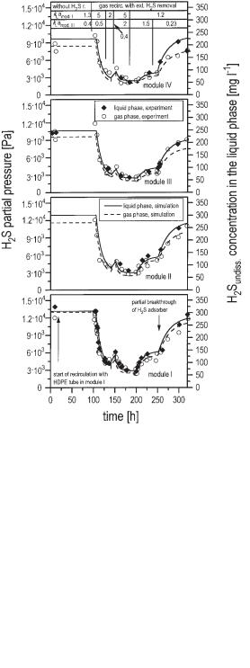
Applying Eqs. 32–34 to each module of the biogas tower reactor and paying additional regard to the liquid mixing, which is described in Section 6.4.1, the H2S content in the liquid phase and the gas phase in the different sections of the reactor can be simulated as shown in Figure 6.34. It can be seen that the highest concentration of H2S is found in the liquid phase at the bottom of the reactor (module I). The cal-

Fig. 6.34 Effect of recycling biogas on the H2S concentration in the gas phase and the liquid phase in the pilot scale biogas tower reactor. Wastewater was simultaneously supplied to modules I, II, and III. Gas was recycled to module I: 2.3, 13, 5, 13, 1.8, 1.8 m3 h–1 and to module II: 0, 0, 2, 2, 3, 0 m3 h–1 in the sequence of the experiment according to the denoted time intervals; sulfate content of wastewater: 3.4–4.5 g L–1; mean residence time of wastewater in the reactor: 2.1 d), r., recirc. recirculation, ext. external, mod. module.

6.6 Influence of Hydrostatic Pressure on Biogas Production 197

culated kLa values in the pilot scale biogas tower reactor are larger by a factor of about 5–10 than those in the UASB reactor. Therefore, the differences between the liquid and the gas phase concentrations are much smaller. By recirculating biogas using an external H2S adsorber, values as small as 50 mg L–1 undissociated H2S in the reactor liquid can be realized.

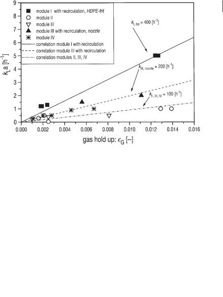
The kLa values identified are proportional to the gas holdup åG in the reactor suspension according to Eq. 35 as shown in Figure 6.35.

The proportional coefficient k depends largely on the size of the bubbles produced. The smallest interfacial area is found when bubbles are generated only by an overflow of the gas collection devices kII = kIII = kIV = 100 h–1. kLa is improved by using a nozzle for the gas injection kIII,nozzle = 200 h–1. In a gas injection over a frit made of high density polyethylene, kI,frit = 400 h–1 is found.

Fig. 6.35 kLa values as a function of gas holdup in the different reactor modules of the pilot scale biogas tower reactor. Gas was supplied to module I by means of a HDPE frit and to module III by means of a simple nozzle.

6.6

Influence of Hydrostatic Pressure on Biogas Production

Knowledge of the effect of higher hydrostatic pressure on the anaerobic digestion is important for the understanding of anaerobic microbiological processes in landfills,

198 6 Modeling of Biogas Reactors

sediments of lakes, or deeper parts of high technical biogas reactors, especially of biogas tower reactors. Anaerobic reactors for the treatment of sewage sludge may also have a height up to 50 m.

In the literature very little has been published on this important effect. The reason may be found in the high complexity of performing experiments under steady-state conditions and elevated pressure. A theoretical and experimental study was published by Friedmann and Märkl (1993, 1994). It was shown that the most important effect of elevated pressure is due to the higher solubility of the product gases, like CO2, H2S, and NH3. According to Eqs. 3–14 the pH may change because of a higher solubility of these gases and, therefore, the equilibrium of dissociation of all the relevant substances will shift, with a significant effect on the kinetics of biogas production.

If a higher percentage of the produced gases is dissolved in the liquid phase of the reactor broth at higher pressures, a smaller amount of gas G will remain compared to the gas volume at a usual pressure of 105 Pa G0. Because this effect is different for each gas component, the composition of the produced biogas will change when increasing hydrostatic pressure.

Assuming the number of gas bubbles remains constant, increasing the pressure leads to a smaller size of bubbles (bubble diameter: dB) according to Eq. 36.

The bubble diameter decreases because the relative content of dissolved gas is higher at higher pressures, which results in a smaller G; furthermore, the pressure phydrost itself reduces the bubble size. Highbie’s penetration theory (Eq. 37) and Stoke’s theory (Eq. 39) of bubble rising velocity (wb) show the influence on the mass transfer coefficient kL (Eq. 40).

It is assumed that the diffusion coefficient D in Eq. 37 is constant at the different pressures and the boundary layer renewal time ô can be calculated according to Eq. 38. Due to the fact that the interfacial contact area a between liquid and gas will also be smaller according to Eq. 41, the kLa value with respect to the hydrostatic pressure phydrost can be calculated by Eq. 42.

6.7 Outlook 199

Altogether at a higher hydrostatic pressure the transport capacity of the product gases from the liquid phase to the gas phase (Section 6.5, Eqs. 32 and 33) decreases and, therefore, the concentration of these gases in the liquid phase will increase additionally.

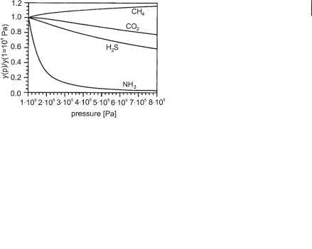
Friedmann and Märkl (1993) give a solution of this complex physicochemical system (39 nonlinear equations have to be solved simultaneously). Figure 6.36 gives an example of the results, showing the relative change in the composition of produced biogas as a function of pressure.

Fig. 6.36 Relative change in the composition of the produced biogas due to an alteration in the absolute pressure (model calculation for the digestion of wastewater of bakers’ yeast production).

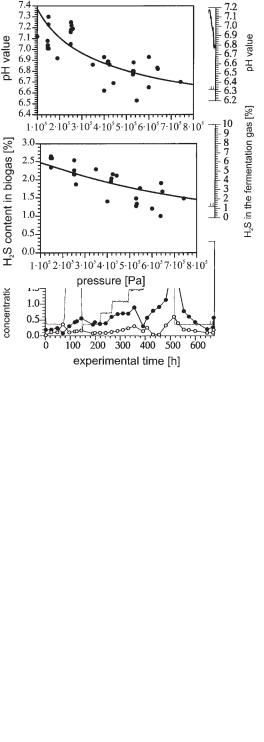
Experiments were performed in a 16 L stirred tank reactor. The reactor was equipped for continuous experiments under elevated pressures (up to 8 · 105 Pa). The pH value, the concentration of undissociated H2S in the liquid, and the H2S content in the gas were measured in situ and continuously. Concentrations of the undissociated acetic acid and propionic acid were also detected (Fig. 6.37).

A comparison of the total experimental data investigated with model calculations is given in Figure 6.38 showing a reasonable degree of agreement.

6.7 Outlook

The mathematical model was developed and its use was demonstrated with the example of a biogas tower reactor. The hydrodynamic and liquid mixing behavior (Section 6.4), as well as the application of the mathematical model for reactor control (Section 6.7) are directly attributed to this reactor type.

But it should also be stated that the structure of the model and the basic understanding of the system behavior are of a more general nature and can be applied to all reactor types. This holds especially true for the measuring techniques (Section 6.2) and the microbial kinetics (Section 6.3). In each biogas reactor the transport of the gas phase (Section 6.5) will plays an important role. The influence of gas oversaturation which is a function of that transport phenomenon, is of particular impor-

200 6 Modeling of Biogas Reactors

Fig. 6.37 Experiments digesting wastewater of bakers’ yeast production at different pressures (pressure difference to normal pressure) in a stirred tank reactor (active volume 16 L). Continuous feeding of wastewater (TOC = 12 g L–1, concentration of sulfate 2.8 g L–1). Pressure was kept constant

b 2500 Pa within a certain time interval to achieve steady state conditions.

a)

b)

Fig. 6.38a, b Comparison between model calculation and experiment. a pH as a function of the absolute pressure, b H2S content in the biogas as a function of the absolute pressure.