Environmental Biotechnology - Jordening and Winter

122 4 Modeling of Aerobic Wastewater Treatment Processes

Models are no better than the assumptions upon which they are built. Several factors influence their behavior. The way they handle detailed wastewater composition is important. Wastewater characterization has a strong impact on real plant behavior as well as on its modeling. Errors in characterization of the wastewater or changes in the composition of the wastewater can result in erroneous modeling results.

4.3

Elements of Activated Sludge Models

An activated sludge model consists of various elements:

•transport processes

•components

•biological and chemical processes

•hydraulics

To this can be added a framework of component conversion and data presentation tools. The amount of detail needed depends on the intended use of the model and on the amount of information available on the wastewater and the treatment plant.

4.3.1

Transport Processes and Treatment Plant Layout

Transport processes deal only with movement of water and do not include any chemical or biological processes. The flow scheme of the treatment plant, which describes the movement of water and sludge, must be known, and a model of the flow scheme must be part of the overall model. Often it is necessary to simplify the flow scheme, due to a high complexity of the plant or to limitations to the number of tanks that can be applied in the model. Simplification of a flow scheme can be very beneficial for improving the overview of the situation in the plant. Parallel tanks can be modeled as one tank, and tanks in series might also be modeled as one. However, one must be aware that the more simplified the flow scheme model is, the greater the model calculations may deviate from the real world.

The flow pattern of wastewater and sludge must be known. Not all treatment plant operators can give this information directly, at least not correctly.

4.3.1.1 Aeration

Aeration in each of the tanks must be described, either with a fixed oxygen concentration or as an aeration coefficient, KLa, operating uncontrolled or controlled together with a control strategy. Aeration of tanks without mechanical aeration should also be taken into account. The oxygen penetration through the surface of, e.g., denitrification tanks can be significant.

The use of a fixed oxygen concentration is a simplification that does not allow for simultaneous nitrification–denitrification processes to be modeled, nor the impact

4.4 Presentation of Models 123

of oxygen in recycle flows. Thus, the KLa model is recommended for professional modeling.

4.3.1.2Components

Components are the soluble and suspended substances that one wants to model, including substances present in the raw wastewater as well as substances found within the treatment plant. The components to model depend on the purpose of the model. If the purpose is to model a nitrifying plant, one phosphorous component will suffice, but if modeling of biological phosphorous removal is the objective, then at least two phosphorous components are needed: polyphosphate in the biomass (XPP) and a soluble component, orthophosphate (SPO4).

4.3.1.3Processes

Processes include modeling of chemical and biological processes. The model to be used is always a strong simplification of reality, but these simplified models often give reasonable modeling results, but sometimes not. For example, a simple phosphorous precipitation model, like the one applied in ASM2 (Henze et al., 1995), can model the part of phosphorous removal that is not related to assimilation and biological excess uptake. On the other hand, a model that does not account for the denitrification that occurs in nitrification tanks, the so-called simultaneous denitrification, gives effluent nitrate concentrations that are too high. Thus, the degree of simplification must be considered. If one wants to model denitrification, there must be at least one process for this (anoxic growth of heterotrophic biomass). But it is also possible to apply many processes for the description of denitrification. This occurs for a model that is aimed at predicting intermediates like nitrite, dinitrogen oxide, nitrous oxide, etc., in the denitrification process.

4.3.1.4Hydraulic Patterns

The hydraulics of the various tanks have to be modeled. Any tanks can be modeled as ideal mixing, but some may need to be modeled as a series of ideally mixed tanks. More complex models of the hydraulics are seldom needed.

4.4

Presentation of Models

The complex interrelationship between the various components and processes are best presented in a matrix. A very simple model for an activated sludge process for removal of organic matter is shown in the matrix in Table 4.1. With this table it is possible to obtain a quick overview of the conversions in the described process.

1244 Modeling of Aerobic Wastewater Treatment Processes

Table 4.1. Simple model matrix for activated sludge organic removala.

aSO2: soluble oxygen, g O2 m–3; SS: soluble organic substrate, g COD m–3; XH: biomass, g COD m–3; YH: yield coefficient, g COD g–1 COD; mm,H : maximum growth rate, d–1; KS: half saturation constant, g COD m–3; bH: decay constant, d–1.

4.4.1

Mass Balances

The rows in the matrix give the mass balance of the process. The second row in Table 4.1 shows, e.g., that decay removes biomass, XH (the stoichiometric coefficient is negative, –1), and produces soluble substrate, SS (the stoichiometric coefficient is +1).

4.4.2

Rates

The rate equations of the processes are found in the right column (Table 4.1). To find the rate for the change in biomass in relation to decay, rXH, the rate equation must be multiplied by the stoichiometric coefficient in the matrix; that is:

4.4.3

Component Participation

The columns in the matrix (Table 4.1) give an overview of which processes the various components participate in (according to the model). The second column shows that the substrate, SS, is removed by aerobic growth and is produced by decay.

4.5

The Activated Sludge Models Nos. 1, 2 and 3 (ASM1, ASM2, ASM3)

Most models for activated sludge processes are based on the IAWQ Activated Sludge Model No. 1, called ASM1 (Henze et al., 1987). This model is used as a platform for further model development and is today the international standard for advanced ac-

4.5 The Activated Sludge Models Nos. 1, 2 and 3 (ASM1, ASM2, ASM3) 125

tivated sludge modeling. Because the ASM contains only a very simplified model, most modelers expand the ASM1, depending on the degree of complexity needed to model the actual problem. In some situations more complex kinetic equations are needed, in others more processes or more components have to be included. Nutrient limitation of the growth processes is usually included.

4.5.1

Activated Sludge Model No. 1 (ASM1)

The ASM1 model describes activated sludge processes with nitrification and denitrification. It is the experience of more than 10 years of use that the model gives a good description of the processes, as long as the wastewater has been characterized in detail and is of domestic or municipal origin. The model was not developed to fit industrial wastewater treatment. When used for industrial wastewater, great care should be taken in calibration and in interpretation of the results.

The ASM1 can calculate several details in the plant:

•oxygen consumption in the tanks

•concentration of ammonia and nitrate in the tanks and in the effluent

•concentration of COD in the tanks and in the effluent

•MLSS in the tanks

•solids retention time

•sludge production

As with all models, ASM1 also gives erroneous results if it is fed erroneous or overly simplified information. Table 4.2 shows the process matrix for ASM1. All processes, reaction kinetics, mass balances, and stoichiometry in the model are included in the matrix. If understood, the matrix notation is a useful tool to obtain an easy overview of the model.

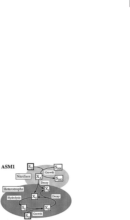
In the ASM1 the processes for organic matter removal and nitrification are slightly coupled, as seen in Figure 4.1.

Fig. 4.1 Processes for heterotrophic and nitrifying bacteria in the Activated Sludge Model No. 1 (ASM1) (Gujer et al., 1999).

1284 Modeling of Aerobic Wastewater Treatment Processes

4.6

Wastewater Characterization

Wastewater characterization is an important element in dealing with models. The detailed wastewater composition has a significant influence on the performance of the treatment processes (Henze, 1992). The degree of detail needed in the wastewater characterization depends on the objective of modeling. Figure 4.3 shows a detailed fractionation of municipal wastewater in relation to biological phosphorous removal. As can be seen, what is considered ‘soluble’ in the model (substances with the symbol S) is not equivalent to analytically determined soluble material, because part of the particulate organic material is easily degradable. Thus, from a reaction point of view, it cannot be distinguished from the analytically soluble material.

Table 4.3 shows a detailed fractionation of wastewater, which allows for modeling denitrification as well as biological phosphorous removal processes.

The characterization of wastewater can be simplified by combining existing data on BOD, COD, soluble fractions, etc. An example of this is from the Dutch river boards, which use the procedure shown below (Roeleveld and Kruit, 1998).

Influent:

where SI = soluble COD (0.1 ìm filter) in the effluent from a low loaded biological treatment plant.

Table 4.3. Wastewater components in ASM2. Note that modeled levels of soluble organic material are higher than analytically determined levels.

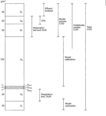
4.6 Wastewater Characterization 129

COD fractionation in the Activated Sludge Model No. 2 (ASM2). The figure shows a typical composition of primary settled municipal wastewater. Various analytical methods that can be used for the determination of single components are shown. Organic inert suspended material, XI, and organic, slowly degradable suspended material, XS, can be determined only by modeling and calculation (Henze et al., 1995). At present, no methods exist to directly determine these two fractions independently. For inert suspended organic matter, XI, the reason is that its concentration in the sludge originates in two sources: it is a component of the raw wastewater and is also produced during the decay of microorganisms. These two contributions cannot be separated analytically at present. Slowly degradable suspended organic matter, XS, cannot be determined analytically except from calculation based on determinations of the other fractions of organic matter.

130 4 Modeling of Aerobic Wastewater Treatment Processes

SS + XS is determined from a BOD5 measurement or from a BOD20 measurement (or calculation):

A simplified evaluation of the nitrogen components is done based on the content of nitrogen in the organic components:

where fNX and fNS are the fractions of nitrogen (g N g–1 COD) and are typically around 0.03 g N g–1 COD (Henze et al., 1997).

4.7

Model Calibration

Calibration of models is difficult. It is mandatory for a successful calibration that the content and the functioning of the model be understood. When calibrating by hand, it is important to follow a strategy and be aware of which parameters are to be used for which part of the calibration. It is equally important to know the realistic intervals within which the various parameters should vary, in order to still have a realistic model. Table 4.4 shows the steps to follow for calibration of the Activated Sludge Model No. 1. Constants not shown should, under normal circumstances, not be changed.

For processes without changes in performance or loading, calibration is easy but not very reliable. Often, many sets of calibration constants give a nice model fit. The

Table 4.4. Calibration steps for the activated sludge model no. 1 (ASM1).