

Environmental Biotechnology - Jordening and Winter
.pdf6.4 Hydrodynamic and Liquid Mixing Behavior of the Biogas Tower Reactor 181
the concentration of total acetic acid. It can be seen that the behavior changes completely if it is compared to the graph in Figure 6.12. Adding H2S to the fermentation broth changes the kinetics from a Michaelis–Menten type to a substrate inhibition type. The effect can be explained by the continuous decrease of the pH value if the concentration of acetic acid is increased. At smaller values of pH more of the total hydrogen sulfide exists in the form of undissociated H2S and the inhibitory effect increases along the abscissa.
6.4
Hydrodynamic and Liquid Mixing Behavior of the Biogas Tower Reactor
Mixing of the liquid phase with respect to the scale-up of a reactor has to be known to understand the nutrient supply of all of the active reactor regions and to avoid local overloading of the reactor. The biogas tower reactor of Figure 6.1 consists of four modules. The active volume of one reactor unit, as shown in Figure 6.2, is 280 m3 (height 25 m, diameter 3.5 m). A settler at the top of the reactor helps to maintain high biomass concentrations within the reactor.
The principal function of one module is described in Figure 6.18. Biogas produced below this module rises and is collected under the collecting device (1), where it can be withdrawn. The quantity of gas withdrawn is controlled by a valve (2). If less gas is taken off than collected, the remaining gas rises through the open cross-sec- tional area (3) into the next module and into the next gas collecting device (5). The baffle (4) separates the space between two gas collecting devices into two channels joining at the top and the bottom of each module. Because of the rising gas on one side of the baffle, there is a difference in the gas holdup in two channels, which corresponds to a fluid circulation along the baffle (Blenke, 1985). The upflow channel is
Fig. 6.18 One module of the BTR (1,5: gas collecting devices; 2,6: gas control units; 3,7: connecting cross-sectional areas; 4: baffle).
182 6 Modeling of Biogas Reactors
called a “riser” and the downflowing part is called a “downcomer”. The circulation velocity is strongly linked to the amount of gas passing through the open cross-sec- tional area (3). Hence, by controlling the gas outlets (2) and (6) it is possible to control the liquid circulation velocity and the mixing time in a module. If no gas is withdrawn, both the circulation velocity and the mixing intensity are high. In contrast, if all collected gas is withdrawn, the circulation slows and good settling conditions for biomass set in. In the lower zones of the reactor it might be advantageous to support the mixing characteristics, in the higher zones good settling conditions should be established. As in mixing within one module, the mixing between two neighboring modules depends, as experiments show, on the gas flow rate through the open cross-sectional area ( 3) between the two modules. If gas rises through this area, turbulence is generated, causing a convective transport between the two modules. If the gas flow rate through the connecting area (3) is low, the mass transport between the modules decreases.
6.4.1
Mixing of the Liquid Phase
Reinhold et al. (1996) provided a theoretical and analytical analysis of the mixing behavior of a BTR. Experiments were performed on a laboratory (Fig. 6.19) and a pilot
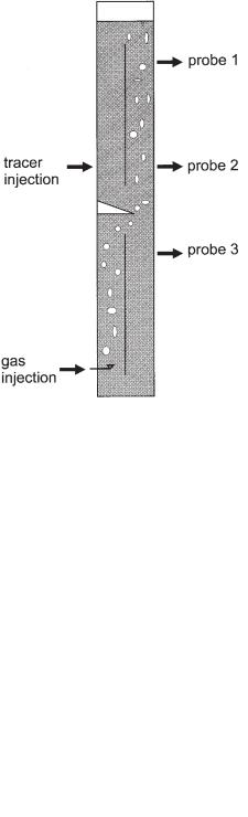
Fig. 6.19 Laboratory reactor representing a model of two modules of the BTR. It was filled with 0.1% ethanol in tap water, and air was injected through a sparger at the bottom to simulate biogas production (height: 6.5 m; diameter 0.4 m; volume 0.7 m3; height of a module 3.5 m; length of the baffle 2.89 m).
6.4 Hydrodynamic and Liquid Mixing Behavior of the Biogas Tower Reactor 183
scale (Fig. 6.20). To study mixing, a saline solution was injected in the form of a Dirac impulse as a tracer at positions indicated in Figures 6.19 and 6.20. The time course of the salt concentration was continuously monitored by conductivity probes at different positions. For the experiments the reactors were filled with tap water. To reduce the coalescence of bubbles and to obtain small bubbles as observed in biogas reactors, 0.1% ethanol was added. Instead of biological gas production, air was injected at the bottom of the reactors. It was assumed that the dominating effect on the circulating flow was caused by gas coming from the lower module. The results of the experiments can be summarized as follows. The mixing times for a 95% homogeneity after a tracer impulse are
•mixing within one module: (1–2) · 102 s
•mixing from one module to a neighboring module: (0.5–2) · 103 s
Because the heights of a module in the laboratory and in the pilot scale reactor do not differ much, the situation on the pilot scale is more or less the same as in the laboratory scale reactor.
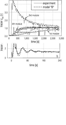
Mixing within one module due to the axial dispersion in the circulating flow is shown in Figure 6.21, presenting laboratory scale experiments. The concentration profiles over time for the four modules of the pilot scale reactor after applying a Dirac impulse in the third module are recorded in Figure 6.22. The experimental behavior is simulated very well by a mathematical model.
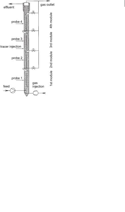
Fig. 6.20 Pilot scale BTR (height 20 m; diameter 1 m; volume 15 m3; height of a module 4 m; length of the baffle 3 m).
184 6 Modeling of Biogas Reactors
Fig. 6.21 Mixing of a Dirac impulse in the upper module of the laboratory scale reactor (Fig. 6.19).
Fig. 6.22 Mixing of a Dirac impulse (3rd module) in the pilot scale BTR (Fig. 6.20).
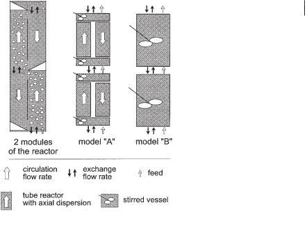
The structure of the mathematical model developed is shown in Figure 6.23. The structures of the two models A and B follow the modular structure of the reactor
concept. Both models couple two neighboring modules by the flow of the feed
·
(V feed), which is constant within the tower reactor and is directed from the bottom to the top of the reactor. The central idea of both models is to predict the coupling
between two modules by the so-called “exchange flow rate”. This virtual flow rate
·
(Vexchange) accounts for the situation of a turbulent exchange of volume elements in
the area between two modules (A exchange). This turbulent flow is driven by the bub-
·
bles passing this area. V feed is kept at zero during the experiment. Also, in reality the
·
contribution of V feed is usually small compared to the turbulent exchange flow
·
Vexchange.
6.4 Hydrodynamic and Liquid Mixing Behavior of the Biogas Tower Reactor 185
Fig. 6.23 Structure of models A and B as compared to the BTR for describing the mixing behavior of the liquid phase.
6.4.1.1Model A
Model A, which is a more detailed one, is able to describe mixing within a module as well as intermixing between modules. Each module is composed of four compartments. Riser and downcomer are mathematically replaced by tube reactors with axial dispersion. At the bottom and the top of each module, riser and downcomer join
in mixing zones which are regarded as stirred vessels. The four zones are linked by
·
the circulation flow rate Vcirc. Since the cross-sectional area of the riser A riser and the
·
downcomer A downc. as well as the flow rate through the riser Vriser and the down-
·
comer Vdownc. are equal, the mean circulation velocity wm is given by Eq. 19.
· |
|
· |
|
||
|
Vriser |
|
Vdownc. |
(19) |
|
wm = Ariser |
= |
Adownc. |
|||
|
|||||
Each real module of the reactor is thus replaced by a “ring structure” of four reactors. The transport and mixing mechanisms in this ring structure are convection and axial dispersion. The mathematical equations of model A can be derived from the mass balances of each of the four compartments. Model A needs three parame-
ters for calculating the mixing behavior: the liquid circulation velocity wm, the axial
·
dispersion coefficient Dax, and the exchange rate Vexchange. All these parameters depend on the gas flow rate entering the module from the lower module. For more details of the model, the mathematical structure, and the procedure of solving the partial differential equations, the publication of Reinhold et al. (1996) should be consulted.

186 6 Modeling of Biogas Reactors
6.4.1.2 Model B
Model B, which is simpler, consists of only one stirred vessel per module (Fig. 6.23). This model is able to describe the mixing behavior of the whole reactor if the mixing intensity within one module is high compared to the tracer transport from one module to another. This assumption holds true in the real situation, as shown earlier. Model B links the stirred vessels in the same way as model A. The intermixing
·
between two neighboring modules is again modeled by an exchange flow rate V ex- change going up and down. Eq. 20 shows the material balance for one module i.
|
dci |
· |
· |
· |
|
|
Vi |
= Vexchange, i–1 (ci –1 – ci) + Vexchange, i (cic1–ci) + V feed (ci –1 – ci) |
(20) |
||||
dt |
||||||
|
|
|
|
|
||
For describing the mixing of one compound in a BTR with model B, the number of ordinary differential equations is equal to the number of modules. It is an initial-
value problem which can be solved by the Runge–Kutta method. The only necessary
·
parameter for calculating the mixing behavior is the exchange flow rate Vexchange.
Experiments in both laboratory and pilot scale reactors are carried out at different
·
gas flow rates Vgas to investigate the dependence of the hydrodynamic parameters on the gas loading. Although there are many investigations on airlift loop reactors and bubble columns in general, the results cannot be applied to this type of reactor because the gas and liquid loading of the BTR are far below those of the airlift loop and bubble column reactors found in the literature. Since the present BTR has
unique characteristics, it was necessary to determine the exchange flow rates
·
Vexchange. Consequently, studies on the circulation velocity wm and the axial disper-
sion Dax were carried out.
·
The characteristic parameters Dax, wm, Vexchange, are a function of the gas loading of the system. The parameters can be obtained by using the least-squares method to fit the simulation to the experimental data. The results are shown in Figures 6.24–6.26.
In Figure 6.24 the axial dispersion coefficient is plotted against the superficial gas velocity of the riser uriser which is given by Eq. 21.
·
uriser = Vgas (21) A riser
This coefficient was only determined on the laboratory scale. Figure 6.25 shows the mean circulation velocity wm of the laboratory scale and the pilot scale reactors as a function of the superficial gas velocity of the riser uriser, From a momentum balance the mean circulation velocity wm can be calculated on the basis of the difference in gas holdup between riser and downcomer Äå and the knowledge of the total pressure loss (friction) coefficient î according to Eq. 22.
wm = ; |
2 g L |
Äå |
(22) |
|
|||
|
|
|
|
6.4 Hydrodynamic and Liquid Mixing Behavior of the Biogas Tower Reactor 187
Fig. 6.24 Axial dispersion coefficient as a function of the superficial gas velocity in the riser.
Fig. 6.25 Mean circulation velocity of the liquid as a function of the superficial gas velocity of the riser.
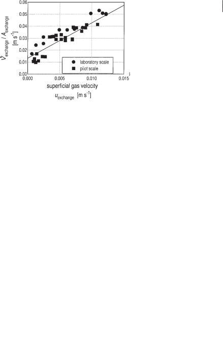
Fig. 6.26 Effect of the superficial gas velocity on the exchange flow rate between two modules.

188 6 Modeling of Biogas Reactors
L is the length of the baffle and g is the gravitational acceleration. The gas holdup can be correlated from the superficial gas velocity uriser according to Weiland (1978). Due to experiments of Reinhold et al. (1996), it can be calculated according to Eqs. 23 and 24).
Äå = 0.27 uriser0.8 |
(laboratory scale) |
(23) |
Äå = 0.76 uriser0.8 |
(pilot scale) |
(24) |
The pressure loss coefficients were determined to be î = 6.9 on the laboratory scale and to be î = 4.8 on the pilot scale. As expected, the total friction coefficient î
slightly decreases during scale-up.
·
Figure 6.26 shows the exchange flow rate Vexchange as a function of the superficial gas velocity uexchange, which can be calculated according to Eq. 25.
·
uexchange = Vgas (25) A exchange
It is quite remarkable that the findings of Figure 6.26 are invariant with the scale
·
of the reactor. Because Vexchange dominates the mixing behavior of the system (indeed, it is the only experimental parameter necessary for model B) this result is very important for the scale-up of biogas tower reactors.
6.4.2
Distribution of Biomass within the Reactor
The wastewater is passing the BTR from the bottom to the top of the reactor. With this feeding procedure the upflow velocity due to the feed increases – at a constant mean residence time of wastewater in the reactor – linearly with the height of the reactor. Therefore, in high reactors it is essential to have reliable mechanisms to retain the active biomass. These mechanisms and the resulting distribution of biomass within the reactor were studied by Reinhold and Märkl (1997).
6.4.2.1 Experiments
Experiments were performed with a two-modular laboratory tower reactor (height 6.5 m) and in a pilot scale tower reactor (height 20 m) as shown in Figure 6.2 and described in Table 6.1. The laboratory tower reactor was filled with tap water and anaerobic pelletized sludge. The sludge was biologically, inactive, as no substrate was present in the tap water, i.e., it did not produce any fermentation gas. Air was injected at the bottom of the column instead of real biogas. As the reactor was built out of transparent material, visual observations were possible in addition to measurements from samples. The following observations were made during these experiments:
•The suspended solids concentration in the lower module is always higher than in the upper module.
6.4 Hydrodynamic and Liquid Mixing Behavior of the Biogas Tower Reactor 189
·
• The macroscopic liquid turbulence backmixing flow (Vexchange), which causes the interaction between adjoining modules, was visualized through the movement of the sludge pellets as indicated by the arrows (7) in Figure 6.27.
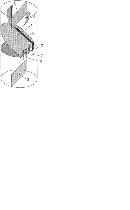
• The most remarkable observation is also indicated in Figure 6.27: At the lower end of the baffle (4) the suspension turns 180° (6) and from this flow a continuously downward-directed solid mass flow (5) is observed, falling at the downward-slop- ing flat blade (1) and from there sliding to the module below. This may prove to be a very effective mechanism of retaining active sludge in the reactor.
Measurements of sludge distribution were also performed in the pilot scale tower reactor digesting wastewater of the bakers’ yeast company. The BTR was inoculated with pelletized sludge, and the space loading was increased in 75 d to 8.8 kg TOC m–3 d–1 with a TOC removal efficiency of 60%. The TOC conversion rate by the sludge was 1.2 kg TOC (kg SS)–1 d–1. The size of the pellets in the reactor ranged from 0.08 to 1 mm. Volatile suspended solids were about 50%–60% of the suspended solids. Elementary analysis showed that 50% of the dry matter was carbon. Two main observations concerning the sludge distribution were made during these experiments on the pilot scale:
•There is no difference in the concentration of suspended solids between riser and downcomer. Each module can be regarded as a completely mixed reactor.
•The concentration of suspended solids in the BTR decreases gradually in upward direction from module to module.
Fig. 6.27 Flows in the coupling zone of two adjacent modules: (1) gas collecting device; (2) connecting area between
the modules; (3) upper end of the lower baffle; (4) lower |
|
|
· |
end of the upper baffle; (5) sedimenting mass flow (Msedi); |
|
· |
· |
(6) circulating flow (Vcirc); (7) backmixing flow (Vexchange);
·
(8) feed flow (Vfeed).
1906 Modeling of Biogas Reactors
6.4.2.2 Mathematical Modeling
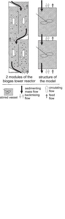
The structure of the mathematical models is shown in Figure 6.28. The mass balance of one module (i), including the interaction with an upper (i + 1) and a lower module (i–1), leads to Eq. 26.
|
dSSi |
· |
|
· |
|
|
|
|
|
Vi |
= V exchange,i–1 (SSi –1–SSi) +Vexchange,i (SSic1–SSi) |
|
|
||||||
dt |
(26) |
||||||||
|
|
|
|
|
|
||||
|
|
· |
· |
· |
· |
|
|||
|
|
|
Vi SSi |
||||||
|
|
+ V feed (SSi–1–SSi) – Msedi,i –1 + Msedi,i + Mprod |
|
|
|
||||
|
|
|
n |
||||||
− Vk · SSk
kp1
In this equation Vi denotes the volume of a module, SSi the concentration of sus-
· ·
pended solids, V feed, the volumetric feed rate of the reactor, and Msedi,i the sediment-
·
ing mass flow between the modules. The produced biomass M prod according to the growth of organisms could be calculated according to the TOC consumed (Eq. 27).
· ·
M prod = 0.1 · V feed (TOCin – TOCout )
·
The volumetric exchange flow Vexchange, i measurements in Figure 6.26.
(27)
is calculated with Eq. 28 on the basis of
Fig. 6.28 Structure of the mathematical model compared to two modules of the BTR.