

The Physics of Coronory Blood Flow - M. Zamir
.pdf260 8 Elements of Unlumped-Model Analysis
|
x |
p(x) |
|
||
|
|
|
|
|
p0(x0) |
|
p1(x1) |
|||
|
|
|
|
|
|||
|
|
|
|
|
|
|
|
|
|
|
|
|
|
|
|
|
|
|
|
|
|
x1 |
|
|
|
|
|
|
|
||
|
|
|
|
|
|
|
|
|
|
|
|
|
|
x1=l1 |
|
x0=0 |
|
|
|
||||
|
|
x0=l0 |
|||||
|
|
|
|
x1=0 |
|||
Fig. 8.3.1. In unlumped-model analysis the pressure p in a tube is considered as a function of streamwise position coordinate x measured from the tube entrance. In a sequence of tube segments in series, the pressure and the position coordinate are re-defined in each tube segment and are confined to that tube only.
It is important to note that the domain of p0 is restricted to the first tube segment only, and the domain of p1 is restricted to the second tube segment only. Thus, p1(0) is a function of x1 only, and p1(0) is the value of p1 at x1 = 0 with no ambiguity. Similarly, p0 is a function of x0 only, and p0(0) and p0(l0) are values of p0 at x0 = 0 and at x0 = l0, respectively, again without ambiguity.
Eqs. 8.3.5, 8 then give
p1(0) = p0(0) − |
8μ |
(8.3.9) |
πa04 ql0 |
which indicates how the pressure at the beginning of the second tube segment is determined by the pressure at the end of the first tube segment. Using this result in Eq. 8.3.6, we find that the pressure at any point within the second tube segment is then determined by
p1(x1) = p0(l0) − |
8μ |
(8.3.10) |
πa14 qx1 |
These expressions can be generalized in a straightforward way, so that in the presence of a third tube segment we would have
p2(0) = p1 |
(0) − |
8μ |
(8.3.11) |
|||
|
|
ql1 |
||||
πa14 |
||||||
p2(x2) = p1 |
(l1) − |
|
8μ |
(8.3.12) |
||
|
|
qx2 |
||||
πa24 |
||||||

8.3 Steady Flow along Tube Segments |
261 |
and in general, if there are n + 1 segments,
pn(0) = pn−1(0) − |
8μ |
(8.3.13) |
||||
|
|
|
qln−1 |
|||
πan4 |
−1 |
|||||
pn(xn) = pn−1(ln−1) − |
|
8μ |
(8.3.14) |
|||
|
|
qxn |
||||
|
πan4 |
|||||
It is convenient to put these expressions in nondimensional, normalized forms, using properties of the first tube segment as reference properties. Thus, the position coordinates in each tube segment are normalized by writing
X0 = x0 (8.3.15) l0
X1 = |
x1 |
(8.3.16) |
|
l1 |
|||
. |
|
||
|
|
||
. |
|
|
|
. |
xn |
|
|
Xn = |
(8.3.17) |
||
ln |
|||
|
|
so that, in terms of the new position coordinate X, the normalized length of each tube segment is now 1.0.
The magnitude of the pressure drop in the first tube segment is given by
|Δp0| = |
|p0(l0) − p0(0)| |
(8.3.18) |
||
= |
|
8μ |
ql0 |
(8.3.19) |
|
4 |
|||
|
|
πa0 |
|
|
and this quantity is now used to define a nondimensional form of the pressure in each tube segment, namely
P0 |
(X0) = |
p0(x0) − p0(0) |
(8.3.20) |
|
|Δp0| |
||||
|
|
|
||
|
= −X0 |
(8.3.21) |
||
and the nondimensional pressures at the two ends of the first tube segment are then given by
P0(0) |
= 0 |
(8.3.22) |
P0(1) |
= −1 |
(8.3.23) |
Similarly, the pressure in the second tube, in nondimensional form, is now defined and given by

262 8 Elements of Unlumped-Model Analysis
P1(X1) = |
p1(x1) − p0(0) |
|
|
|
|
|
|
|
|
|
|
|
|
|
|
|
|
|
|
|
||||||||||||||||||
|
|
|
|
|
|
|
|Δp0| |
|
|
|
|
|
|
|
|
|
|
|
|
|
|
|
|
|
|
|
|
|
|
|
|
|||||||
|
= |
p0(l0) − p0(0) |
|
− |
a0 |
|
|
4 |
x1 |
|
|
|||||||||||||||||||||||||||
|
|
|
|
|
|
|Δp0| |
|
|
|
|
|
a1 |
|
|
|
l0 |
|
|||||||||||||||||||||
|
= P0(1) − |
a1 |
|
4 |
l0 |
X1 |
|
|
|
|
|
|||||||||||||||||||||||||||
|
|
|
|
|
|
|
|
|||||||||||||||||||||||||||||||
|
|
|
|
|
|
|
|
|
|
|
|
|
|
|
a0 |
|
|
|
|
|
|
|
l1 |
|
|
|
|
|
|
|
|
|
|
|
|
|
||
|
= −1 − |
a1 |
4 |
l0 X1 |
|
|
|
|
|
|
|
|
||||||||||||||||||||||||||
|
|
|
|
|
|
|
|
|
|
|
||||||||||||||||||||||||||||
|
|
|
|
|
|
|
|
|
|
a0 |
|
|
|
|
|
|
l1 |
|
|
|
|
|
|
|
|
|
|
|
|
|
|
|||||||
and at the two ends of the tube |
|
|
|
|
|
|
|
|
|
|
|
|
|
|
|
|
|
|
|
|
|
|
|
|
|
|
|
|
|
|
|
|
|
|
||||
|
P1(0) = −1 |
|
|
|
|
a1 |
|
4 |
l0 |
|
|
|
|
|
|
|
|
|||||||||||||||||||||
|
P1(1) = −1 − |
|
|
|
|
|
|
|
|
|||||||||||||||||||||||||||||
|
|
|
|
|
|
|
|
|
|
|
||||||||||||||||||||||||||||
|
|
|
|
|
|
|
|
|
|
|
|
|
|
|
|
a0 |
|
|
|
|
|
|
l1 |
|
|
|
|
|
|
|
|
|
|
|||||
|
|
|
|
|
|
|
|
|
|
|
|
|
|
|
|
|
|
|
|
|
|
|
|
|
|
|
|
|
|
|
|
|
|
|||||
In the presence of a third tube, we find |
|
|
|
|
|
|
|
|
|
|
|
|
|
|
|
|
|
|
|
|
||||||||||||||||||
P2(X2) = |
p2(x2) − p0(0) |
|
|
|
|
|
|
|
|
|
|
|
|
|
|
|
|
|
|
|
|
|
|
|
|
|
|
|||||||||||
|
|
|Δp0| |
|
|
|
|
|
|
|
|
|
|
|
|
|
|
|
|
|
|
|
|
|
|
|
|
|
|
|
|
|
|
|
|||||
= |
p1(l1) − p0 |
(0) |
|
|
|
|
|
|
a0 |
|
|
|
4 |
x2 |
|
|
|
|
|
|
|
|
||||||||||||||||
|
|
|
|
|
|
|
|
|
|
|
− |
|
|
|
|
|
|
|
|
|
|
|
|
|
|
|
|
|||||||||||
|
|
|Δp0| |
|
|
|
|
|
a2 |
|
l0 |
|
|
|
|
|
|
|
|
|
|
||||||||||||||||||
= P0(1) − a1 |
|
4 |
l0 |
X1 |
|
|
|
|
|
|
|
|
|
|
|
|
|
|||||||||||||||||||||
|
|
|
|
|
|
|
|
|
|
|
|
|
|
|
||||||||||||||||||||||||
|
|
|
|
|
|
|
a0 |
|
|
|
|
|
|
|
|
l1 |
|
|
|
|
|
|
|
|
|
|
|
|
|
|
|
|
|
|
|
|
||
|
|
|
|
|
|
|
|
|
|
|
|
|
|
|
|
|
|
|
|
|
|
|
|
|
|
|
|
|
|
|
|
|
|
|
|
|
|
|
= −1 − |
a1 |
4 |
l0 |
|
− |
|
a2 |
4 |
l0 X2 |
|||||||||||||||||||||||||||||
|
|
|
|
|
||||||||||||||||||||||||||||||||||
|
|
|
|
|
a0 |
|
|
|
|
|
l1 |
|
|
|
|
|
|
|
|
|
a0 |
|
|
|
|
|
l2 |
|
||||||||||
and in general |
|
|
|
|
|
|
|
|
|
|
|
|
|
|
|
|
|
|
|
|
|
|
|
|
|
|
|
|
|
|
|
|
|
|
|
|
|
|
Pn(Xn) = −1 − a1 |
4 |
l0 − a2 |
4 |
l0 |
− . . . |
|||||||||||||||||||||||||||||||||
|
|
|
||||||||||||||||||||||||||||||||||||
|
|
|
a0 |
|
|
|
|
|
|
|
l1 |
|
|
|
|
|
|
|
|
a0 |
|
|
|
|
|
|
|
|
l2 |
|
||||||||
|
|
|
|
|
|
|
|
|
|
|
|
|
|
|
|
|
|
|
|
|
|
|
|
|
|
|
|
|
|
|
|
|
|
|
|
|
|
|
− an |
4 |
l0 |
Xn |
|
|
|
|
|
|
|
|
|
|
|
|
|
|
|
|
|
|
|
|
|||||||||||||||
|
|
|
|
|
|
|
|
|
|
|
|
|
|
|
|
|
|
|
|
|
||||||||||||||||||
|
|
a0 |
|
|
|
|
|
ln |
|
|
|
|
|
|
|
|
|
|
|
|
|
|
|
|
|
|
|
|
|
|
|
|
|
|
|
|
|
|
(8.3.24)
(8.3.25)
(8.3.26)
(8.3.27)
(8.3.28)
(8.3.29)
(8.3.30)
(8.3.31)
(8.3.32)
(8.3.33)
(8.3.34)
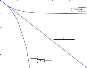
The results indicate that in this convenient nondimensional form, the pressure distribution along a sequence of tube segments in series consists of a series of linear pressure drops, with the pressure starting from a normalized value of 0 at entry and dropping linearly to −1 at the end of the first tube. Subsequent values of the pressure depend on the lengths and diameters of subsequent tubes. If, for the purpose of illustration, it is assumed that the
8.3 Steady Flow along Tube Segments |
263 |
tube lengths are proportional to their diameters, the pressure distribution in each tube segment becomes dependent on the ratios of radii only, namely
P1(X1) = −1 − |
a1 |
|
3 |
X1 |
|
|
|
|
(8.3.35) |
||||
|
|
|
|
|
|||||||||
|
|
a0 |
|
|
|
|
|
|
|
|
|
|
|
P2(X2) = −1 − |
a1 |
|
3 |
− |
a2 |
|
3 |
|
|
(8.3.36) |
|||
|
X2 |
|
|
||||||||||
|
|
a0 |
|
|
|
|
a0 |
|
|
|
|
|
|
. |
|
|
|
|
|
|
|
|
|
|
|
|
|
. |
|
|
|
|
|
|
|
|
|
|
|
|
|
. |
|
|
|
3 |
|
|
|
|
3 |
|
|
3 |
|
Pn(Xn) = −1 − |
a1 |
|
− |
a2 |
|
an |
|||||||
|
− . . . − |
Xn (8.3.37) |
|||||||||||
|
|
a0 |
|
|
|
|
a0 |
|
|
|
a0 |
|
|
If it is assumed further, for the purpose of illustration again, and for reasons to become apparent in the next section, that the radii of successive tube segments are diminishing such that
|
|
a0 |
= |
a1 |
= |
a2 |
. . . = 21/3 |
(8.3.38) |
|
|
|
|
|
|
|||||
|
|
a1 |
a2 |
a3 |
|
|
|||
then these results become |
|
|
|
|
|
|
|||
P1 |
(X1) = −1 − (2)1X1 |
|
(8.3.39) |
||||||
P2 |
(X2) = −1 − (2)1 − |
(2)2X2 |
(8.3.40) |
||||||
|
. |
|
|
|
|
|
|
|
|
|
. |
|
|
|
|
|
|
|
|
|
. |
|
|
|
|
|
|
|
|
Pn(Xn) = −1 − (2)1 − |
(2)2 − . . . − (2)nXn |
(8.3.41) |
|||||||
and if, for the purpose of comparison, the radii of successive tube segments are increasing, such that
|
a0 |
|
|
a1 |
|
|
|
|
a2 |
|
|
|
|
1 |
|
1/3 |
|
|
|
|
|
|
|
|
= |
|
= |
|
|
. . . = |
|
|
|
|
|
|
|
(8.3.42) |
|||||||
|
a1 |
a2 |
a3 |
2 |
|
|
|
|
|
|||||||||||||
we find |
|
|
|
|
|
|
|
|
|
|
|
|
|
|
|
|
|
|
|
|
|
|
P1(X1) = −1 |
− |
1 |
|
1 |
|
|
|
|
|
|
|
|
|
|
|
|
(8.3.43) |
|||||
|
|
|
X1 |
|
|
|
|
|
|
|
|
|
|
|||||||||
2 |
|
|
|
|
|
|
|
|
|
|
|
|||||||||||
P2(X2) = −1 |
− |
1 |
|
1 |
|
|
1 |
|
2 |
|
|
|
|
|
|
|
(8.3.44) |
|||||
|
|
|
− |
|
X2 |
|
|
|
|
|
||||||||||||
2 |
|
2 |
|
|
|
|
|
|||||||||||||||
. |
|
|
|
|
|
|
|
|
|
|
|
|
|
|
|
|
|
|
|
|
|
|
. |
|
|
|
|
|
|
|
|
|
|
|
|
|
|
|
|
|
|
|
|
|
|
. |
|
|
|
|
|
|
|
1 |
|
|
|
|
2 |
|
|
|
|
|
|
|
|
|
Pn(Xn) = −1 |
− |
1 |
|
|
|
1 |
|
|
|
|
|
1 |
|
n |
(8.3.45) |
|||||||
|
|
|
− |
|
− . . . − |
|
Xn |
|||||||||||||||
2 |
|
2 |
2 |
|||||||||||||||||||
In the trivial case where successive tube segments have the same diameters, the results are clearly
264 8 Elements of Unlumped-Model Analysis
P1(X1) = −1 |
− X1 |
(8.3.46) |
|
P2(X2) = −1 |
− 1 |
− X2 |
(8.3.47) |
. |
|
|
|
. |
|
|
|
. |
|
|
|
Pn(Xn) = −1 |
− 1 |
− 1 − . . . − Xn |
(8.3.48) |
These results are illustrated graphically in Fig. 3.8.2, where it is seen that the above trivial case serves as a good reference in which the pressure distribution in each tube segment is linear and dropping by the same amount, namely −1. In the case where the radii of successive tube segments are diminishing, the drops in pressure in successive segments increase very rapidly, and the reverse happens when the radii of successive tube segments are increasing. While these examples are fairly artificial, they serve as useful guides when considering branching tubes.
streamwise distance X (normalized)
|
00 |
2 |
4 |
6 |
8 |
10 |
P(X) |
-2 |
|
|
|
|
|
|
|
|
|
|
|
|
pressure |
-4 |
|
|
|
|
|
|
|
|
|
|
|
|
nondimensional |
-6 |
|
|
|
|
|
-8 |
|
|
|
|
|
|
|
|
|
|
|
|
|
|
-10 |
|
|
|
|
|
Fig. 8.3.2. Pressure distribution in steady flow along a sequence of tube segments in series. The streamwise distance X here is a cumulative coordinate along the sequence of tube segments whereby the normalized length of each tube segment is 1.0. Thus, the first tube segment extends from X = 0 to X = 1.0, the second extends from X = 1.0 to X = 2.0, etc. If the radii of successive tube segments are increasing, the pressure drops very rapidly, while if the radii are decreasing the pressure drops very slowly. In the trivial case where the radii of successive tube segments remain unchanged, the pressure drops by the same amount (−1.0) in each tube segment, with this case serving as a useful reference for comparison.
8.4 Steady Flow Through a Bifurcation |
265 |
8.4 Steady Flow Through a Bifurcation
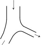
It is well established that the underlying design of arterial pathways in the cardiovascular system is that of an open tree structure, and the same is true in the coronary circulation. In an open tree structure (Fig. 1.6.1) a root vessel segment divides into branches, then each branch in turn divides into new branches, etc. It has been determined that the number of branches at each division is almost invariably two, that is, the tree structure is formed by repeated bifurcations as shown schematically in Fig. 1.6.1. This tree structure is termed “open” in the sense that there are no cross-connections between the branches, so that the path from the root segment to any other vessel segment within this structure is unique. The issue of possible cross-connections (collateral vessels) in the coronary circulation was discussed in Section 1.6 and will not be considered further. In this section we consider only open tree structures, in which the building block from which the tree is constructed is an arterial bifurcation.
We begin by considering an arterial bifurcation, being modelled by three tube segments as shown schematically in Fig. 8.4.1. Subscripts 0,1,2 are used to identify the parent and the two branch segments, respectively, as shown in the figure, with the convention that subscript 1 shall always be used to identify the branch with the larger diameter. With the flow being from parent to branches, conservation of mass requires that flow rate q0 in the parent vessel be equal to the sum of the flow rates in the two branches, that is
q0 = q1 + q2 |
(8.4.1) |
q0
q2
 q1
q1
Fig. 8.4.1. Arterial trees in the cardiovascular system are formed largely by repeated bifurcations whereby a vessel segment divides into two branches and then each of the branches in turn divides into two branches, etc. The same is true in the coronary circulation. An arterial bifurcation is shown here schematically, with the parent vessel identified by subscript 0 and the two branches by subscripts 1, 2, with the convention that subscript 1 is always reserved for the branch with the larger radius. Flow rate q0 in the parent vessel is divided into q1, q2 in the branches.

266 8 Elements of Unlumped-Model Analysis
The pressure distribution under conditions of steady flow through the bifurcation can be considered by following two streamwise paths: one from parent to branch-1 and another from parent to branch-2. Along each path the situation is the same as that of two tubes in series, as considered in the previous section. It is important to emphasize again that here too we assume that the idealized conditions of fully developed Poiseuille flow prevail along the full length of each tube segment, ignoring local deviations at the two ends of each segment. The justification for this is that we are interested primarily in the pressure distribution along the tubes forming the bifurcation rather than in the local details of the flow field within the bifurcation. The only di erence here is that, because of flow division, the flow rates in consecutive tube segments are not the same. Along the path from the root segment to the first branch, we may then return to Eqs. 8.3.5, 6 in the previous section and, using the same notation as in the previous section, write
p0(x0) = p0(0) − |
8μ |
(8.4.2) |
|
|
q0x0 |
||
πa04 |
|||
p1(x1) = p1(0) − |
8μ |
(8.4.3) |
|
|
q1x1 |
||
πa14 |
|||
For pressure continuity at the bifurcation point we have, as in the previous section,
p1(0) = p0(l0) |
(8.4.4) |
thus Eq. 8.4.3 for the pressure distribution along the path to branch-1 becomes
p1(x1) = p0(l0) − |
8μ |
(8.4.5) |
πa14 q1x1 |
and, similarly, the pressure distribution along the path from the root segment to branch-2 is then given by
p2(x2) = p0(l0) − |
8μ |
(8.4.6) |
πa24 q2x2 |
The lengths of the three vessel segments can be normalized by defining new normalized coordinates
X0 |
= |
x0 |
(8.4.7) |
|
|
l0 |
|||
|
|
|
|
|
X1 |
= |
x1 |
(8.4.8) |
|
|
l1 |
|||
|
|
|
|
|
X2 |
= |
x2 |
(8.4.9) |
|
|
l2 |
|||
|
|
|
|
|
In terms of these coordinates, the normalized length of each of the three vessel segments is now 1.0, which, as we see shortly, is useful for plotting the pressure distributions along the paths to the two branches using the same scale
8.4 Steady Flow Through a Bifurcation |
267 |
regardless of their di erent lengths. Furthermore, these pressure distributions can now be put in nondimensional form by using the properties of the parent tube segment as reference properties. In particular, the magnitude of the pressure drop in the parent tube segment, namely
|Δp0| = |
|p0(l0) − p0(0)| |
(8.4.10) |
||
= |
|
8μ |
q0l0 |
(8.4.11) |
|
4 |
|||
|
|
πa0 |
|
|
is used to put the pressure distributions in nondimensional forms, that is
P0(X0) = |
p0(x0) − p0(0) |
|
|
|
|
(8.4.12) |
|||||||||||||||
|
|
|
|
|
|
|
|
|Δp0| |
|
|
|
|
|
|
|
|
|
||||
|
|
= −X0 |
|
|
|
|
|
|
|
|
|
|
|
|
(8.4.13) |
||||||
P1(X1) = |
p1 |
(x1) − p0(0) |
|
|
|
|
|
|
|
|
|
|
|
|
(8.4.14) |
||||||
|
|
|
|
|
|
|
|
|
|
|
|
|
|||||||||
|
|
|Δp0| |
|
|
|
|
|
|
|
|
|
|
|
|
|
|
|
|
|
||
|
p0 |
|Δp0| |
|
|
|
|
− a1 |
|
4 |
q0 |
l0 |
|
|||||||||
|
|
|
|
|
|
|
|
||||||||||||||
= |
(l0) − p0(0) |
|
|
|
|
a0 |
|
|
|
|
q1 |
x1 |
(8.4.15) |
||||||||
|
|
|
|
|
|
|
|
|
|
|
|
|
|
|
|
||||||
= −1 − a1 |
|
4 |
q0 |
l0 |
X1 |
|
|
(8.4.16) |
|||||||||||||
|
|
|
|||||||||||||||||||
|
|
|
a0 |
|
|
|
|
|
|
q1 |
|
|
|
l1 |
|
|
|
|
|
|
|
P2(X2) = |
p2 |
(x2) − p0(0) |
|
|
|
|
|
|
|
|
|
|
|
|
(8.4.17) |
||||||
|
|
|
|
|
|
|
|
|
|
|
|
|
|||||||||
|
|
|Δp0| |
|
|
|
|
|
|
|
|
|
|
|
|
|
|
|
|
|
||
|
p0 |
|Δp0| |
|
|
|
|
− a2 |
|
4 |
q0 |
l0 |
|
|||||||||
|
|
|
|
|
|
|
|
||||||||||||||
= |
(l0) − p0(0) |
|
|
|
|
a0 |
|
|
|
|
q2 |
x2 |
(8.4.18) |
||||||||
|
|
|
|
|
|
|
|
|
|
|
|
|
|
||||||||
= −1 − a2 |
|
4 |
q0 |
l0 |
X2 |
|
|
(8.4.19) |
|||||||||||||
|
|
|
|||||||||||||||||||
|
|
|
a0 |
|
|
|
|
|
|
q2 |
|
|
|
l2 |
|
|
|
|
|
|
|
If it is assumed that vessel lengths are proportional to their radii, the pressure distributions along the two paths become
P1(X1) = −1 − |
a1 |
|
3 |
q0 |
X1 |
(8.4.20) |
||
|
||||||||
|
|
a0 |
|
|
|
q1 |
|
|
P2(X2) = −1 − |
a2 |
|
3 |
q0 |
X2 |
(8.4.21) |
||
|
||||||||
|
|
a0 |
|
|
|
q2 |
|
|
Furthermore, in the theory of vascular branching it is found that a power law relation exists between the radius of a blood vessel and the average flow rate which the vessel is destined to carry, that is
268 8 Elements of Unlumped-Model Analysis
q aγ |
(8.4.22) |
where γ shall be referred to as the “power law index”. If this relation is used in Eqs. 8.4.20, 21, the pressure distributions become
P1(X1) = −1 − |
a0 |
|
3−γ |
(8.4.23) |
|
X1 |
|||
a1 |
||||
P2(X2) = −1 − |
a0 |
|
3−γ |
(8.4.24) |
|
X2 |
|||
a2 |
If the power law relation between radius and flow rate is used also in Eq. 8.4.1, then the relation between the three flow rates at a bifurcation becomes a relation between the three radii of the vessels involved, namely
a0γ = a1γ + a2γ |
(8.4.25) |
Essentially, this relation dictates that if one daughter branch at a bifurcation has a comparatively large radius then the other must have a comparatively small one. This is clearly a reflection of the conservation requirement in Eq. 8.4.1, namely that if one branch carries a relatively larger proportion of the flow then the other must carry a correspondingly small proportion. The relation between the radii can be seen more clearly by introducing a “bifurcation index”
α = |
a2 |
(8.4.26) |
|
a1 |
|||
|
|
Recalling that in our convention branch-1 is always the branch with the larger radius, except when the two radii are equal, this index is a measure of the asymmetry of a bifurcation in terms of the relative radii of its two branches. Its value is 1.0 when the bifurcation is perfectly symmetrical, meaning that its two branches have the same radii, and close to zero when the bifurcation is highly asymmetrical, meaning that one of the two branches has a much larger radius than the other. Thus α has the convenient range of values of 0 to 1.0 for the entire spectrum of possible bifurcations.
The relation between the three radii in Eq. 8.4.25, after division by a1 or a2, can now be put in terms of the bifurcation index α, that is
a0 |
= (1 + αγ )1/γ |
(8.4.27) |
||||
a1 |
||||||
|
|
|
|
|
||
a0 |
= |
1 + αγ |
|
1/γ |
|
|
|
(8.4.28) |
|||||
a2 |
αγ |
|
||||
Using these diameter ratios in Eqs. 8.4.23, 24, finally, gives the following expressions for the pressure distributions
8.4 |
Steady Flow Through a Bifurcation 269 |
|||
P1(X1) = −1 |
− (1 + αγ ) γ3 −1 |
(8.4.29) |
||
|
|
+ αγ |
γ3 −1 |
|
P2(X2) = −1 |
− |
1 |
|
(8.4.30) |
αγ |
||||
A considerable volume of work on arterial branching has gone into analysis of the optimal design of arterial bifurcations which, as we see here, depends primarily on the value of the power law index γ in the relation between the radius of a vessel and the flow rate which that vessel is destined to carry (Eq. 8.4.22). Three values in particular were considered on theoretical grounds, namely γ = 2, 3, 4, while vessel diameters actually measured in the cardiovascular system have produced values of γ highly scattered within and beyond this theoretical range [220]. A key consideration in determining the “optimum” value of γ is the shear stress τw which blood flow exerts on endothelial tissue and which under the idealized conditions of Poiseuille flow is given by
du |
r=a |
|
τw = μ dr |
(8.4.31) |
streamwise distance X (normalized)
|
00 |
0.5 |
1 |
1.5 |
2 |
P(X) |
-0.5 |
|
P0 |
|
|
|
|
|
|
|
|
pressure |
-1 |
|
|
|
|
-1.5 |
|
|
|
|
|
nondimensional |
|
|
|
|
|
|
|
|
|
P1 |
|
-2 |
|
|
|
|
|
|
P0 |
|
|
|
|
-2.5 |
|
|
|
P2 |
|
|
|
P2 |
|
|
|
|
|
P1 |
|
|
|
|
-3 |
|
|
|
|
|
|
q a2 |
|
|
|
|
|
|
|
|
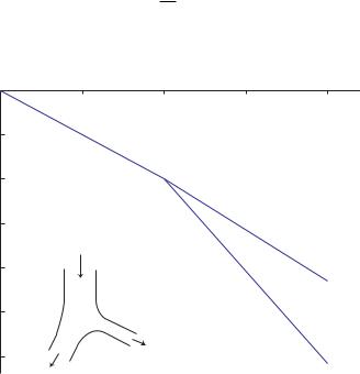
Fig. 8.4.2. Pressure distributions within the three vessel segments forming an arterial bifurcation, under the idealized conditions of steady Poiseuille flow and on the assumption of a power law relation between the radius of each vessel and the flow rate through it. If the power law index is less than 3, as it is here, the pressure drop in the branch with the smaller radius (branch-2) is higher than that in the other branch.