

The Physics of Coronory Blood Flow - M. Zamir
.pdf280 8 Elements of Unlumped-Model Analysis
e ect simultaneously at every position along the tube. As the input pressure rises, fluid responds by an appropriate increase in flow rate, and while this rise in flow rate is somewhat delayed because of fluid inertia, the delay is the same everywhere along the tube.
r
 u(r,t)
x
r |
|
c |
|
|
|
|
x |
u(x,r,t) |
|
|
Fig. 8.6.1. Pulsatile flow in a rigid tube, where flow moves in tandem all along the tube (top), compared with pulsatile flow in an elastic tube where flow is in the form of a wave (bottom). In the elastic tube, a rise in pressure is first absorbed by a bulging in the tube wall and then transmitted downstream as the pressure falls and the tube recoils. Thus, in oscillatory flow where the input pressure rises and falls repeatedly, a wave motion is created within the tube. The “wave speed” c is the speed with which the wave progresses downstream.
If the tube is elastic, by contrast, as the input pressure rises, the rise is initially absorbed by a local bulge in the tube wall and is therefore not immediately sensed by fluid in other regions of the tube. Only as the input pressure begins to fall does the bulge in the tube wall begin to recoil and the pressure di erence driving the flow begins to rise and the flow rate responds accordingly [124, 221]. But by this point in time in the oscillatory cycle the input pressure begins to rise again and the cycle is repeated again and again. The result is a “delayed messaging” of the oscillatory input pressure to the rest of the tube, compared with the instant messaging which occurs in a rigid tube.
The most important result of this di erence is that pulsatile flow in an elastic tube produces wave motion along the tube (Fig. 8.6.1), which is strictly analogous to the wave motion observed when the calm surface of a lake is disturbed to cause a local change in pressure. In the latter circumstance the local change in pressure is absorbed locally by a rise of a body of fluid against gravity, which then falls back in analogy with the recoiling of the elastic tube, sending the message along the lake surface.
The speed with which a local change in pressure is transmitted downstream in pulsatile flow in an elastic tube is known as the “wave speed”, appropriately so because it corresponds to the speed with which the bulges in the tube

8.6 Pulsatile Flow in an Elastic Tube |
281 |
wall, like the crests on the surface of a lake, move downstream (Fig. 8.6.1). If the material of the tube wall is perfectly elastic, and if it can be assumed further that the tube wall is “thin” compared with the tube radius, then an approximate expression for the wave speed, known as the Moen-Korteweg formula, is given by
c0 = |
Eh |
(8.6.1) |
ρd |
where E is a measure of elasticity of the tube wall, known as Young’s modulus, or modulus of elasticity, h is the thickness of the tube wall, d is tube diameter, and ρ is the density of the fluid which is assumed constant. The measure of elasticity of the tube wall is such that higher values of E represent increased rigidity of the tube wall. The formula thus indicates that the wave speed is higher in a more rigid tube. An important limit is that in which the tube wall is infinitely rigid, that is it lacks any elasticity at all, in which case the value of E is infinite and therefore the wave speed c0 is infinite. Thus, the “instant messaging” in a rigid tube referred to earlier can now be viewed as messaging occuring at infinite speed, and the di erence between pulsatile flow in an elastic tube and that in a rigid tube can now be re-stated by saying that in a rigid tube wave propagation occurs at infinite speed, hence a change in pressure is sensed instantaneously everywhere along the tube. More accurately, wave propagation is actually absent in a rigid tube because the wave itself is absent, it simply does not materialize.
The two assumptions on which the Moen-Korteweg formula is based, namely that the tube wall is thin and perfectly elastic, can be dealt with by modified forms of the formula. In most general applications, however, these modifications are not required and the formula provides a reasonable approximation as it stands.
A more important aspect of the Moen-Korteweg formula is that it has been derived under conditions of inviscid flow, where the flow does not satisfy the condition of “no-slip” at the tube wall. To satisfy this important physical condition and thereby include the e ects of fluid viscosity a full solution of the equations governing the movements of both the fluid and the tube wall is required. The mathematical problem thus becomes considerably more complicated than that in a rigid tube. The problem has been solved, however, and in what follows we use the main elements of the results [145, 208, 8, 46, 125, 221].
In general, while pulsatile flow in a rigid tube is governed critically by the value of the frequency parameter Ω, pulsatile flow in an elastic tube is governed similarly by the value of Ω but also by the value of the wave speed c which in turn depends on Ω as well as on tube properties. We now distinguish between the wave speed c based on a full solution of the problem, including the e ects of viscosity, and the inviscid wave speed c0 provided by the MoenKorteweg formula in Eq. 8.6.1. The full solution of the problem provides the following relation between the two

8.6 Pulsatile Flow in an Elastic Tube |
283 |
|
1.5 |
|
|
|
|
|
(normalized) |
1 |
|
|
|
|
|
|
|
|
|
|
|
|
wave speed |
0.5 |
|
|
|
|
|
|
|
|
|
|
|
|
complex |
0 |
|
|
|
|
|
|
|
|
|
|
|
|
|
−0.50 |
2 |
4 |
6 |
8 |
10 |
|
|
|
frequency parameter Ω |
|
|
|
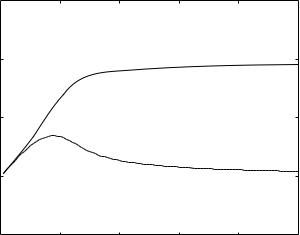
Fig. 8.6.2. The real (solid) and imaginary (dashed) parts of the wave speed c in oscillatory flow in an elastic tube, normalized in terms of the wave speed c0 in inviscid flow which is purely real. For values of the frequency parameter Ω above 3 or so, the real part of c approaches the value of c0 and the imaginary part of c approaches zero, thus c e ectively becomes the same as c0.
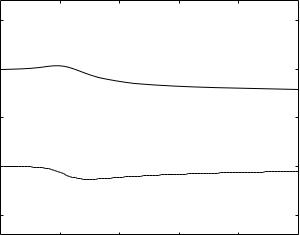
the corresponding expressions for flow in a rigid tube (Eqs. 8.5.19, 24) indicates that one di erence between the two is embodied in what may be referred to as the “elasticity factor” G. Numerical values of G can be found elsewhere [221] and are shown graphically in Fig. 8.6.3, where it is seen that G is a complex quantity whose real part is close to 1.0 and its imaginary part is close to 0.
Another di erence between the expressions for pulsatile flow in an elastic tube and those in a rigid tube is the presence of the streamwise coordinate x in the exponential part of the expressions for an elastic tube. This indicates that in the elastic tube oscillations in pressure and flow occur not only in time as they do in a rigid tube, but also in space, which is the hallmark of wave motion. In a rigid tube where the fluid everywhere along the tube moves in unison there is no wave motion, the entire bulk of the fluid moves back and forth together. In an elastic tube this is no longer the case because there are now oscillations along the tube as indicated by the presence of the streamwise coodinate x in the exponential part of Eqs. 8.6.5–7, which is now eiω(t−x/c) instead of eiωt.
To see the characteristics of the wave motion more clearly we note that
eiω(t−x/c) = eiωt × e−iωx/c |
(8.6.9) |
The first term on the right represents oscillations in time t as for flow in a rigid tube, and the second represents oscillations in x. At a fixed position

8.6 Pulsatile Flow in an Elastic Tube |
285 |
In this form of these expressions it is seen that the extent to which space oscillations modify the flow properties in pulsatile flow in an elastic tube depends critically on the ratio x/λ appearing in the exponential terms on the right. In a tube of length l, maximum e ect clearly occurs at x = l, thus the maximum modifications of the flow depend on the ratio of wave length to tube length, λ/l. To estimate these modifications we may consider a tube in which the wall thickness to diameter ratio h/d is 1/10, the fluid density ρ is 1.0 gm/cm3, and Young’s modulus E is 107 dynes/cm2. Inserting these values in the Moen-Korteweg formula gives an estimate of the inviscid wave speed
c0 = |
Eh |
|
(8.6.14) |
ρd |
|||
10 m/s |
(8.6.15) |
||
The corresponding wave length, at a fundamental frequency f0 of 1 cycle/s, is then
λ0 = |
|
c0 |
|
(8.6.16) |
|
f0 |
|||
|
|
|
||
|
10 m |
(8.6.17) |
||
We use subscript 0 for λ to indicate that here it is based on c0 and f0. The values of both c0 and λ0 above are high because they are based on inviscid flow but they serve as useful benchmarks. Actual values measured in the cardiovascular system may be closer to one half of these values.
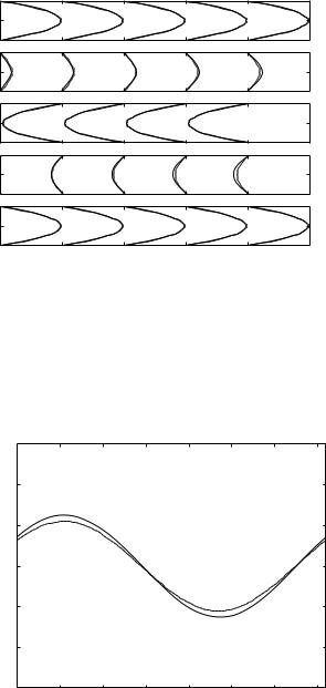
In a coronary artery of length 5 cm, therefore, the ratio of tube length to wave length is approximately 1/100, and comparison of the flow properties with this value are shown in Figs. 8.6.4, 5.
The radial velocity of the tube wall in pulsatile flow in an elastic tube matches the fluid velocity at the inner surface of the tube, that is at r = a, and from Eqs. 8.6.4, 12 and Eq. 8.5.14 we then have
vφ(x, a, t) |
|
2aω |
|
|
|
|
uˆs |
|
= |
iΛ2c |
(1 |
− Gg)eiωt e−i2πx/λ |
(8.6.18) |
and substituting for Λ (Eq. 8.5.13), this simplifies further to
vφ(x, a, t) |
|
2 |
|
|
|
|
uˆs |
|
= |
Rc |
(1 |
− Gg)eiωt e−i2πx/λ |
(8.6.19) |
where Rc is a Reynolds number based on the wave speed c, namely
Rc = |
ρac |
(8.6.20) |
||
μ |
|
|||
|
|
|||
Plots of the normalized radial velocity scaled in terms of 2/Rc, that is plots of (vφ(x, a, t)/uˆs)/(2/Rc) are shown in Fig. 8.6.5. Because of the scaling,
288 8 Elements of Unlumped-Model Analysis
common observation that when the wave reaches the shore or other obstacle such as a boat, it is partially or totally reflected, producing a wave moving in the opposite direction. This backward moving wave then combines with the forward moving wave to produce a complex pattern of wave motion.
The same scenario occurs in an elastic tube, though it is not as clearly visible. In this case a propagating wave may be reflected because of an occlusion or narrowing within or at the end of the tube, or a local change in its elasticity. Any of these will act as an obstacle in the way of a propagating wave and thus act as a reflection site. The most important reflection sites in coronary blood flow and in blood flow in general are vascular junctions. They are important because of their very large number. Vascular trees typically consist of many millions of vascular junctions, and any path for blood flow within the tree typically consists of only short tube segments, each terminating at a vascular junction (Figs. 8.5.1, 2). The propagating wave rarely enjoys any significant length of tube free from obstacles, thus wave reflections are ubiquitous in the coronary circulation as they are in the cardiovascular system in general. The e ect of wave reflections from a single vascular junction may be very small, but the cumulative e ect from many thousands or millions of such junctions can be very large. In the lake analogy this is equivalent to a wave being reflected from many boats of di erent sizes and at di erent positions on the lake surface, leading to a highly complex wave pattern. In a vascular tree the result of this complex pattern of forward and backward moving waves is a change in the pressure distribution within the tree, which in turn a ects blood flow within the tree. Wave reflection e ects in the coronary circulation have received little attention in the past despite the significant role they may play in the dynamics of coronary blood flow [5, 219, 164]
The e ects of wave reflections on the pressure distribution within a vascular tree is therefore a key element in the analysis of pulsatile blood flow. Because these e ects are cumulative, coming from many reflection sites within the tree, and because each of these sites is typically positioned at the end of a short tube segment, there are two essential steps in the computation of these e ects. In the first, one considers the e ects of wave reflections in a single tube, and, in the second step, the results are applied to the hierarchy of tube segments in a branching tree structure to calculate the cumulative e ect. We consider the first of these steps in the present section, and the second in the next chapter.
Since the ultimate aim in this work is to deal with a large number of tube segments in a tree structure, the analysis of wave reflections is essentially one dimensional. The detailed analysis of pulsatile flow in an elastic tube considered in the previous section cannot be carried in full to each of many thousands of tube segments in a tree structure. Instead, we take only the main conclusions from that analysis, namely that an oscillatory input pressure applied at the entrance of an elastic tube produces a travelling wave along the tube. This conclusion can in fact be reached alternatively by considering solutions of wave equations instead of the equations on which the results of
8.7 Wave Reflections |
289 |
pulsatile flow in an elastic tube discussed in the previous section are based. In either case, our starting point is that an input oscillatory pressure of the form [221]
pin(t) = p0eiωt |
(8.7.1) |
applied at the entry to an elastic tube, produces a travelling wave within the tube, of the form
P (x, t) = p0eiω(t−x/c) |
(8.7.2) |
where p0 is the constant amplitude of the input wave, ω is the frequency of oscillation, c is the wave speed, t is time, and x is distance along the tube measured from the entrance.
As discussed in the previous section, this travelling wave consists of two oscillations, one in time and one in space. To separate these two oscillations, and to put the pressure in normalized form, we write
|
|
(x, t) = |
|
P (x, t) |
|
|
|
(8.7.3) |
||
|
P |
|
|
|
||||||
|
|
|
p0 |
|
|
|
|
|||
|
|
|
|
|
|
|
|
|
||
|
|
= e−iωx/c × eiωt |
|
(8.7.4) |
||||||
|
|
= p(x)eiωt |
|
|
|
(8.7.5) |
||||
where |
|
|
|
|
|
|
|
|
||
p(x) = e−iωx/c |
|
|
|
(8.7.6) |
||||||
|
|
|
ωx |
|
ωx |
|
|
|||
|
= cos |
|
− i sin |
|
|
|
(8.7.7) |
|||
|
c |
c |
||||||||
Thus, at di erent points in time within the oscillatory cycle and at di erent positions along the tube, the normalized pressure is given by
|
|
|
P (x, t) = cos ω(t − x/c) + i sin ω(t − x/c) |
(8.7.8) |
|
|
= p(x)eiωt |
(8.7.9) |
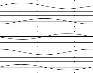
which is a simple cosine or sine function of x, depending on whether we use the real or the imaginary part of the solution. Using the real part, we have a simple cosine wave which progresses along the tube at increasing values of t, as illustrated in Fig. 8.7.1.
The amplitude of this travelling wave represents the peak values of pressure reached at di erent points along the tube and at di erent points in time and
is given by |
|
||
| |
|
(x, t)| = |eiω(t−x/c)| |
(8.7.10) |
P |
|||
|
|
= |p(x)| × |eiωt| |
(8.7.11) |
|
|
= |p(x)| |
(8.7.12) |