The Physics of Coronory Blood Flow - M. Zamir

330 9 Basic Unlumped Models

a tube segment within a tree structure, any departure of the pressure distribution from the “benchmark” of a uniform normalized value of 1.0 provides a direct and useful measure of the e ects of wave reflections in that structure. It is also a highly meaningful measure because the pressure distribution produced by wave reflections in a vessel segment within a vascular tree is superimposed on a pre-existing pressure distribution associated with steady flow within that vessel segment, and the net result is a modified distribution of pressure gradients driving the flow. For the same reasons, the pressure distribution along a vascular tree as a whole has the same utility and functional significance. The focus in this section, therefore, is on determining the pressure distribution within a vascular tree structure under di erent conditions.

We recall from Section 8.7 that an oscillatory input pressure applied at entry to an elastic tube produces a travelling wave within the tube. If this scenario occurs in a tube segment within a vascular tree structure, the travelling wave will progress to the next tube segment within the hierarchy of the tree structure, with the junction point between the two segments usually acting as a wave reflection site because of any di erence in the admittance properties of the two tubes. Typically, only part of the wave will be reflected. The remaining part, usually referred to as the “transmitted” part of the wave, will continue on to the next junction point, and so on. The net result is that the pressure distribution within the tree structure will be modified because of the many reflected waves within the system.

In order to determine the pressure distribution in a branching tree structure, it is necessary to keep track of the “net” pressure wave as it progresses from the root segment of the tree to the periphery, the net pressure wave in each tube segment being the sum of the transmitted wave and any reflected waves. In each tube segment along the way, we use essentially the same analysis as that in Section 8.7 for wave reflections in a single tube, but now the tube position within the tree structure must be identified so that the pressure and flow within it can be mapped along with the pressure and flow within the tree as a whole. For this purpose we use the j, k notation introduced in Section 9.2, whereby j denotes the level of the tree in which a given tube segment is located and k denotes the sequential position of that segment within other segments at that level, as illustrated in Figs. 9.2.3, 4.

Using that notation, the results of Section 8.7 for wave reflections in a single tube can now be placed in the context of a tree structure. In particular, the net pressure wave within a general tube segment at position j, k in a tree structure, using Eqs.8.7.3,19, is now given by

Pj,k (xj,k , t) = p0,j,k eiω(t−xj,k /cj,k ) + Rj,k eiω(t−(2lj,k −xj,k )/cj,k ) (9.6.1)

where lj,k is the length of the tube segment and xj,k is a position coordinate within that length such that the tube segment extends from xj,k = 0 to xj,k = lj,k , Rj,k is the reflection coe cient at the downstream end of the vessel segment, cj,k is the wave speed and p0,j,k is the amplitude of the input

oscillatory pressure at entry to that segment, namely

As was done in Section 8.7, the net pressure wave in Eq. 9.6.1 can now be broken into its oscillatory components in time and space such that

The absolute value of this complex function of x, namely |pj,k (x)|, is what we refer to as the “pressure distribution” in a tube segment within a tree structure, and the map of all such distributions together make up the pressure distribution in the tree as a whole. It is a key property of the propagating pressure wave within each tube segment. It represents the net pressure at a fixed point in time at each point along the segment, including forward and backward moving waves. Also, in view of Eq. 9.6.3, it represents the amplitude of time oscillations in pressure at a fixed position within the tube segment.

In the context of a tree structure, it is seen from Eq. 9.6.4 that the pressure distribution in a vessel segment at position j, k within the tree depends on the wave speed cj,k within that segment, on the reflection coe cient Rj,k at the downstream end of the segment, and on the input pressure amplitude p0,j,k at entry to the tube segment. The way in which each of these is determined is outlined below.

Depending on the desired accuracy, the wave speed in a vessel segment within a tree structure may be taken as the constant Moen-Korteweg wave speed c0 as defined by Eq. 8.6.1 and which depends on properties of that segment only, or it may be taken as the wave speed c as defined by Eq. 8.6.2 based on a solution of pulsatile flow in an elastic tube which depends on properties of the tube as well as on the frequency parameter Ω. For comparison purposes, results based on these two alternatives to be presented below shall be identified by c = c0 and c = c respectively.

The reflection coe cient at the downstream end of a tube segment in a tree structure is determined by the characteristic admittance of that segment and by the e ective admittances of the two branch segments forming the bifurcation at that end, as discussed in Section 9.5. If the position of the vessel segment under consideration is j, k, then the positions of the two branch segments at its downstream end (xj,k = lj,k ) are j + 1, 2k − 1 and j + 1, 2k, as illustrated in Figs. 9.2.3, 4. Using the results of Section 9.5, therefore, Eq. 9.5.20 expressed in the notation of the present section gives for the reflection coe cient

332 9 Basic Unlumped Models

The characteristic admittance Y0 is defined by Eq. 9.5.5 and is determined by the radius of the tube segment and by the wave speed which again may be taken as c or c0 as discussed above, depending on the desired accuracy. The e ective admittance Ye, using Eq. 9.5.22 in present notation, is given by

Finally, the input pressure amplitude p0,j,k at entry to the tube segment at position j, k is obtained by equating the local pressure in all three vessel segments that meet at that point (xj,k = 0), recalling that in a branching tree structure based on repeated bifurcations, three vessel segments meet at entry to and at exit from each interior tube segment, as illustrated in Figs. 9.2.3, 4. For junctions beyond the root level of the tree, that is for j > 0, this gives

For the root segment of the tree where j = 0 the input pressure amplitude p0,0,1 is clearly equal to the amplitude of input pressure to the tree as a whole. That is, if the latter is given by

Note, however, that the oscillatory pressure that actually prevails at the root of the tree is given by

and

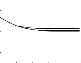
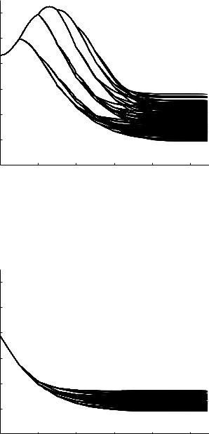
Fig. 9.6.5. Pressure distributions along di erent paths within the 11-level tree model at a frequency of 10 Hz. Comparison with the corresponding results for the 5-level tree model shown in Fig. 9.6.2 indicates clearly that the e ects of wave reflections are larger here, as marked by larger departures from the benchmark of uniform distribution at a normalized value of 1.0 which occurs when wave reflections are absent.

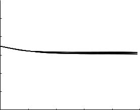
Fig. 9.6.6. Pressure distributions along di erent paths within the 11-level tree model as in Fig. 9.6.5 but here at a frequency of 5 Hz.

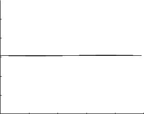
Fig. 9.6.7. Pressure distributions along di erent paths within the 11-level tree model as in Fig. 9.6.5 but here at a frequency of 1 Hz.

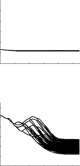
Fig. 9.6.8. Pressure distributions along di erent paths within the 11-level tree model at a frequency of 10 Hz as in Fig. 9.6.5 but here the root segment of the tree has a diameter of 25 mm compared with 4 mm in that figure. Thus the scale of the tree model in this case is representative of the scale of the human systemic arterial tree while that in Fig. 9.6.5 is representative of the coronary arterial tree. Wave-length-to-tube-length ratios are much lower in this case, thus the characteristic highs and lows in the pressure distributions.

Fig. 9.6.9. Pressure distributions along di erent paths within the 11-level tree model as in Fig. 9.6.8, but here at a frequency of 5 Hz which means higher wave lengths and thus higher wave-length-to-tube-length ratios than in that figure.

Fig. 9.6.10. Pressure distributions along di erent paths within the 11-level tree model as in Fig. 9.6.8, but here at a frequency of 1 Hz, which means considerably higher wave lengths and thus considerably higher wave-length-to-tube-length ratios than in that figure.