The Physics of Coronory Blood Flow - M. Zamir

350 9 Basic Unlumped Models

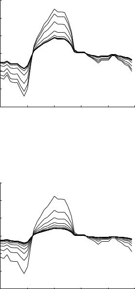
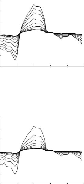
Fig. 9.7.8. Evolution of the composite cardiac pressure wave as it travels down path-1 of the 11-level tree model at a frequency of 10 Hz. The bold curve at the top represents the initial form of the wave as applied at entry while the thin curve above it represents the form of the wave that actually prevails at entry, the two being di erent because of wave reflections returning from downstream. This demonstrates graphically that some local “peaking” occurs initially before the waveform begins to flatten as it progresses further along the hierarchy of the tree and as indicated by subsequent curves in the sequence. Both the local peaking and subsequent flattening is consistent with the corresponding pressure distributions shown in Fig. 9.6.5.

tion of the wave is more gradual at all three frequencies, consistent with the corresponding pressure distributions in Figs. 9.6.8–10.

E ects of using the wave speed c obtained from a solution of pulsatile flow in an elastic tube instead of the constant Moen-Korteweg wave speed on which all the above results are based, are shown in Figs.9.7.17-19. Comparing these with the results in Figs. 9.7.8, 10, 12 which are based on c = c0 indicates that the di erence between the two is unremarkable at all three frequencies.

As for the pressure distribution obtained in the previous section, however, it is important to note that the unique condition of “impedance matching” occurs only when γ = 2 and c = c0 (Fig. 9.6.14). When the more accurate wave speed c is used instead of the Moen-Korteweg wave speed c0, matching is no longer attained and significant wave reflection e ects arise as illustrated in Figs.9.7.21-23.

However, as for the pressure distributions discussed in the previous section, a more significant di erence arises if the hierarchy of branch diameters within the tree is changed from one based on the cube law (γ = 3) to one based on the square law (γ = 2). Under the square law the sum of the cross-sectional areas

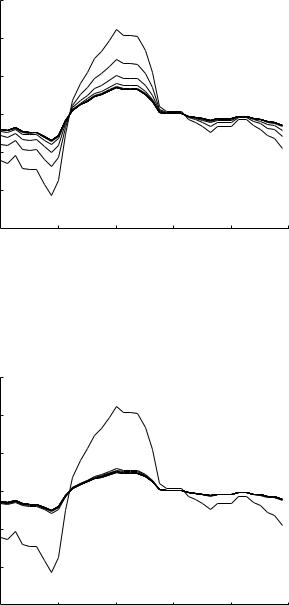
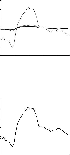
Fig. 9.7.9. Evolution of the composite cardiac pressure wave as it travels down path-2 of the 11-level tree model at a frequency of 10 Hz, which again indicates some initial peaking as in Fig. 9.7.8.

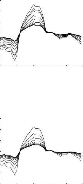
Fig. 9.7.10. Evolution of the composite cardiac pressure wave as it travels down path-1 of the 11-level tree model, as in Fig. 9.7.8 but here at a frequency of 5 Hz, which means higher wave-length-to-tube-length ratios, and hence no peaking in the waveform is observed, consistent with the corresponding pressure distributions in Fig. 9.6.6.

352 9 Basic Unlumped Models

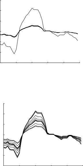
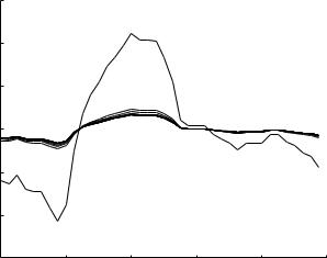
Fig. 9.7.11. Evolution of the composite cardiac pressure wave as in Fig. 9.7.10, but here as it travels down path-2 of the 11-level tree model.

Fig. 9.7.12. Evolution of the composite cardiac pressure wave as it travels down path-1 of the 11-level tree model at the lowest frequency of 1 Hz, which means much higher wave-length-to-tube-length ratios. The abrupt flattening of the waveform is consistent with the pressure distributions in Fig. 9.6.7.

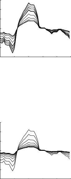
Fig. 9.7.13. Evolution of the composite cardiac pressure wave, as in Fig. 9.7.12, but here as it travels down path-2 of the 11-level tree model.

Fig. 9.7.14. Evolution of the composite cardiac pressure wave as it travels down path-1 of the 11-level tree model at a frequency of 10 Hz as in Fig. 9.7.8, but here the dimensions of the tree are increased to the scale of the systemic circulation, with the root segment of the tree given a diameter of 25 mm compared with 4 mm in that figure. Some initial peaking is observed, consistent with the corresponding pressure distribution in Fig. 9.6.8.

354 9 Basic Unlumped Models

Fig. 9.7.15. Evolution of the composite cardiac pressure wave as it travels down path-1 of the 11-level tree model at a frequency of 5 Hz as in Fig. 9.7.10, but here the dimensions of the tree are increased to the scale of the systemic circulation, with the root segment of the tree given a diameter of 25 mm compared with 4 mm in that figure. Considerably more peaking is observed here while it is completely absent on the scale of the coronary circulation, consistent with the corresponding pressure distribution in Fig. 9.6.9.

Fig. 9.7.16. Evolution of the composite cardiac pressure wave as it travels down path-1 of the 11-level tree model at a frequency of 1 Hz as in Fig. 9.7.12, but here the dimensions of the tree are increased to the scale of the systemic circulation, with the root segment of the tree given a diameter of 25 mm compared with 4 mm in that figure. Peaking is absent in both cases, but the evolution of the wave is considerably more gradual on the systemic scale, clearly because of the lower wave-length-to-tube-length ratios on that scale.

Fig. 9.7.17. Evolution of the composite cardiac pressure wave as it travels down path-1 of the 11-level tree model at a frequency of 10 Hz as in Fig. 9.7.8, but here using the actual wave speed c instead of the Moen-Korteweg wave speed c0 on which the results in that figure are based. The di erence between the two is unremarkable.

Fig. 9.7.18. Evolution of the composite cardiac pressure wave as it travels down path-1 of the 11-level tree model at a frequency of 5 Hz as in Fig. 9.7.10, but here using the actual wave speed c instead of the Moen-Korteweg wave speed c0 on which the results in that figure are based. The di erence between the two is unremarkable.

358 9 Basic Unlumped Models

Fig. 9.7.23. Evolution of the composite cardiac pressure waveform as it travels down path-1 of the 11-level tree model as in Fig. 9.7.21, but here at a frequency of 1 Hz. Impedance matching is not attained at this frequency.

of the two branch segments is equal to the cross-sectional area of the parent segment at all bifurcations within the tree structure. If this is combined with the c = c0 wave speed assumption, then there is no change of admittance as the flow crosses each bifurcation within the entire tree structure, which means that the bifurcations are no longer reflection sites and wave reflections do not arise. Results obtained in the previous section (Fig. 9.6.14) indicated that the pressure distributions obtained under these circumstances are identical with the benchmark of uniform distribution at 1.0, which means, therefore, that the composite pressure waveform would be unchanged as it travels down the tree, a condition known as “admittance matching”. This is indeed the case as illustrated in Fig. 9.7.20. The waveform is unchanged at all levels of the tree and at all three frequencies, consistent with the corresponding pressure distribution in Fig. 9.6.14

9.8 Summary

The ultimate unlumped model of the coronary circulation is unattainable in practice because of the overwhelming details of coronary vasculature and the high degree of variablility in these details from one heart to another, and because of the enormous di culties involved in a study of all aspects of flow in this vasculature. A more modest approach is that of constructing unlumped

models that have only the broad features of scale and branching pattern of coronary vasculature, and to use combinations and variations of these features to probe into the type of dynamics that they can or cannot give rise to, and under what type of conditions.

In order to track the flow in an arterial tree structure it is necessary to identify the position of each vessel segment within that structure. A simple j, k coordinate system can be used for that purpose, whereby the first coordinate identifies the level of the tree in which a vessel segment is located and the second identifies the sequential position of that segment among other segments at that level of the tree. Any path within the tree structure can then be specified in terms of the vessel segments that make up that path, and the pressure distribution along the path can be pieced together from the pressure distributions along each vessel segment. A theoretical tree structure based on a power law with three di erent values of the power law index is used to illustrate this scheme and to find the pressure distributions under steady flow conditions. Because of their uniformity, these theoretical structures do not represent the characteristic heterogenous structure of coronary vasculature, but they serve to illustrate the way in which the pressure varies along the hierarchy of a tree structure.

In pulsatile flow through a rigid tube flow properties depend on the value of the frequency parameter Ω which in turn depends on the tube radius, amongst other things. In a tree structure, therefore, the distribution of the values of Ω within the tree structure is an important determinant of the properties of pulsatile flow along the tree. In general, the value of Ω has its highest value at the root segment of the tree, then decreases from there, along the hierarchy of the tree as the diameters of vessel segments decrease. Peak flow rate and peak shear stress, the maximum values reached within the oscillatory cycle, actually increase from the root segment of the tree towards the periphery because of the decrease in the value of Ω in that direction.

Pulsatile flow in a tree structure consisting of elastic tube segments gives rise to wave propagation and widespread wave reflections because of the large number of vascular junctions. With the ratio of wave length to tube length λ 100 or greater in the coronary circulation as indicated in Fig. 9.4.3, e ects of wave propagation on the flow field are minimal, but the cumulative e ects of wave reflections can be enormous. The aim of the elastic branching tubes model is therefore to establish a method of tracking these reflections and calculating the e ects which they produce in a vascular tree structure consisting of many vascular tube segments and hence many vascular junctions which act as reflection sites.

Pulsatile flow in an elastic tube gives rise to wave propagation within the tube. Impedance is the total opposition to pulsatile flow in an elastic tube, which consists of normal resistance to the steady part of the flow plus opposition to wave propagation. Admittance is the reciprocal of impedance and it represents the extent to which pulsatile flow in an elastic tube is “admitted”, rather than opposed. In a vascular tree structure consisting of elastic tube