The Physics of Coronory Blood Flow - M. Zamir

180 6 Composite Pressure-Flow Relations

and opposition to flow consists of only the resistance R, the corresponding flow wave is given by (Eq. 4.8.7)

As stated in the introduction to this chapter, P (t) is now being used to denote the pressure drop denoted by Δp in earlier chapters, and P0 is a constant representing the amplitude of the pressure wave and denoted by Δp0 in earlier chapters.

It is clear that in this case the relation between the pressure and flow waves is particularly simple. The flow wave has the same form and the same phase angle as the pressure wave, and the amplitude of the flow wave is given by the amplitude of the pressure wave divided by the resistance R, that is

What is important is that this relationship between pressure and flow is fixed, it does not change within the oscillatory cycle. Equally important, however, this relation is only possible when the pressure wave is a simple sine or cosine function. This is clear from the way these solutions were obtained in Chapter 4.

Thus, the relation between pressure and flow cannot be applied to the composite waves of pressure and flow but it can be applied to their individual harmonics because, as we saw in Chapter 5, these harmonics consist of simple sine and cosine waves. Thus, we decompose the pressure wave into its harmonics by writing, as in Chapter 5,

where p1(t) . . . pn(t) are the n harmonics of the oscillatory part of p(t) and p is the (constant) average value of P (t) over one cycle, and if each of these parts of P (t) is now treated separately, we obtain the corresponding series of flow rates, using Eq. 6.2.3,

These components can now be added to give the composite flow wave Q(t) produced by the composite pressure wave P (t), namely

There are two important points to emphasize:

1. The sum in Eq. 6.2.11 to obtain the total Q(t) is only possible because the equation governing Q(t), namely Eq. 4.7.1, is linear.

2.The simple relation in Eq. 6.2.3 between pressure and flow applies only to the components of the pressure and flow waves but not to the composite waves themselves, that is

6.3 Example: Cardiac Pressure Wave

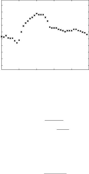
As a first example of pressure-flow analysis, consider the cardiac waveform given numerically in Table 6.3.1 and shown in Fig. 6.3.1. The waveform represents cardiac pressure in mm Hg measured in a 20–kg dog. Note that in this case the pressure data include both the mean and the oscillatory parts of the pressure wave, and we use these below to illustrate the results of the previous section.

To obtain the corresponding flow wave using the scheme outlined in the previous section, the pressure waveform is decomposed into its harmonics as was done in Chapter 5, and the results for the first 10 harmonics are shown numerically in Table 6.3.2. Since the only opposition to flow in this case is the resistance R, then the corresponding harmonics of the flow wave are as in Eq. 6.2.10, namely

However, the resistance R is not known. Since in this section we are only interested in illustrating the analysis involved, we shall use an estimate of R for this purpose.

In the human cardiovascular system, for a 60–kg man, with a cardiac output of 5 L/min and a mean aortic pressure of 100 mm Hg, an estimate of total resistance in the systemic circulation would be

182 6 Composite Pressure-Flow Relations

Fig. 6.3.1. A cardiac pressure wave measured in a 20–kg dog and used as an example to illustrate how the corresponding flow wave is obtained from the given pressure waveform.

If aortic pressure is taken as the input pressure driving flow into the coronary circulation, and if coronary blood flow is estimated at 5% of cardiac output, then an estimate of total resistance in the coronary circulation is

The corresponding estimates for a 20–kg dog, taking the mean cardiac output as 2 L/min, the mean aortic pressure as 100 mm Hg, and coronary blood flow again as 5% of cardiac output, we find

Using the estimated value of R for the coronary system of the dog, and the harmonic components of the cardiac pressure wave in Table 6.3.2, where

Table 6.3.1. A numerical description of the cardiac wave shown in Fig. 6.3.1, giving the pressure (P ) at di erent times t within the oscillatory cycle. The oscillatory period has been normalized to 1.0. The pressure data include both the mean and the oscillatory part of the pressure.

0.000 96.60 0.500 111.00

0.025 96.21 0.525 108.15

0.050 97.27 0.550 103.65

0.075 95.56 0.575 103.00

0.100 95.34 0.600 103.00

0.125 95.38 0.625 103.00

0.150 93.46 0.650 102.00

0.175 91.92 0.675 101.53

0.200 93.88 0.700 101.00

0.225 100.04 0.725 100.26

0.250 104.50 0.750 101.00

0.275 106.68 0.775 101.00

0.300 108.20 0.800 101.00

0.325 110.00 0.825 102.00

0.350 110.95 0.850 102.00

0.375 112.38 0.875 101.13

0.400 113.80 0.900 100.70

0.425 113.00 0.925 99.86

0.450 113.00 0.950 99.47

0.475 112.93 0.975 98.18

184 6 Composite Pressure-Flow Relations

Table 6.3.2. Fourier coe cients of the first 10 harmonics of the pressure wave in Fig. 6.3.1.

where p and q are the mean values of p(t) and q(t) over one oscillatory cycle. For the oscillatory parts of the flow wave, using Eq. 6.3.14 and Table 6.3.2, and taking the period T = 1, we find

≈ 0.0002 × cos (20πt − 127.5263 × π/180) [L/min] (6.3.26)

These components of Q(t) can now be added to give the composite flow wave Q(t) produced by the composite pressure wave P (t), that is

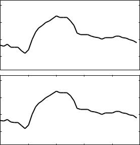
which is shown graphically together with the pressure wave in Fig. 6.3.2.

Fig. 6.3.2. Cardiac pressure wave (top) and corresponding flow wave (bottom) when opposition to flow consists of only resistance R which has been estimated at 1, 000 mm Hg · L/min. We see that in the presence of pure resistance the pressure and flow waves have precisely the same form, the flow wave being only scaled by the value of the resistance R.

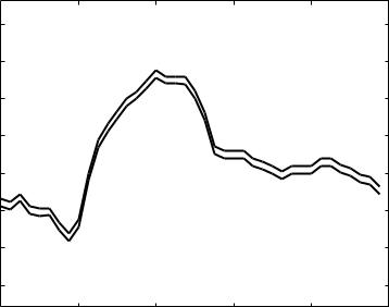
It would be convenient to put the pressure and flow waves together, using the same scale, and the results of this section suggest that in order to do so we should plot P (t) and R × Q(t) (instead of Q(t)), as shown in Fig. 6.3.3. This presentation would be useful not only when the opposition to flow consists of pure resistance but also, and particularly, when other elements of the RLC system are present. In such cases, as we shall see, any small change in the form of the flow wave can be detected more easily and can be attributed directly to inertial (L) or capacitive (C) e ects only, because the e ects of resistance (R) have been scaled out. We shall refer to the product R × Q(t) as the “R-scaled” flow.

186 6 Composite Pressure-Flow Relations

Fig. 6.3.3. When studying pressure-flow relations it is convenient to plot the pressure and flow waves to the same scale so as to compare their waveforms. This can be achieved as seen here by plotting P (t) (solid curve) and the “R-scaled” flow R × Q(t) (dashed) instead of Q(t). When the opposition to flow consists of only resistance R as it is in this case, the two curves become graphically identical. In this figure they are slightly shifted to make them visibly distinct. The use of R-scaled flow is useful also when other elements of the RLC system are present. In such cases any small change in the form of the flow wave can be detected more easily and can be attributed directly to inertial (L) or capacitive (C) e ects only, because the e ects of resistance (R) have been scaled out.

6.4Composite Pressure-Flow Relations Under General Impedance

When opposition to pulsatile flow consists of more than pure resistance, that is, when either inertial or capacitance e ects or both are involved, the relation between a composite flow wave and the corresponding flow wave is more complicated than was seen in the previous section. For the purpose of considering this relation here, the term “impedance” shall be used in a general sense here to mean any form of opposition to flow beyond that of pure resistance.

It is convenient in this and in subsequent sections to use the concept of complex impedance Z introduced in Section 4.9. It was seen in that section that when the opposition to flow consists of only pure resistance, the complex impedance Z becomes real and equal to R, but when any inertial or capacitive

e ects are present, that is any “reactive” e ects, Z is a complex quantity whose real and imaginary parts depend on the nature and arrangement of the reactive elements. In these terms, our interest in this section is in pressure-flow relations when Z has both a real and an imaginary part.

Let the composite pressure wave under consideration be denoted by P (t) and the corresponding flow wave be denoted by Q(t). In Chapter 5 we saw that P (t) can always be separated into a steady part p and a purely oscillatory part, such that

The mean part of the pressure represents the mean value of P (t) over one oscillatory cycle, namely

The oscillation part of the pressure, by definition, has a zero mean. This separation of the composite wave is important because the corresponding flow wave will consist similarly of steady and oscillatory parts, which we shall denote by q and q(t), respectively, and write

The relation between the mean components of the pressure and flow waves, p, q, is fundamentally di erent from that between the oscillatory components, p(t), q(t), and the two relations must be dealt with separately. For the steady components, the relation between pressure and flow is simply that established in Section 6.2, namely

While in Section 6.2 the opposition to flow consisted of only pure resistance, this relation remains valid in this section even though reactive elements are assumed to be present. The reason for this is that reactive e ects come into play only when flow is non-steady. And since here we are able to separate the steady and non-steady parts of the flow, as discussed in Section 6.2, Eq. 6.4.4 can be used for the steady parts of the pressure and flow waves.

One of the most important advantages of using complex impedance is that the relation between the oscillatory parts of the pressure and flow waves can then be put in the general form

However, in this equation the pressure p(t) must be in complex form. And since both p(t) and Z are complex, it follows that q(t) is also complex. Thus, if subscripts r and i are used to denote real and imaginary parts, and we write

wave. Thus Eq. 6.4.5 cannot be applied directly to a composite pressure wave, but it can be applied to its individual harmonics. If there are N harmonics and we denote these by pn(t), then, as we found in Chapter 5, they are given by

and the oscillatory part of the pressure wave is given by

where Mn and φn are (real) constants associated with the Fourier series representation of the composite wave.

Eq. 6.4.5 applies only to each of these harmonics individually, and only if each is considered to be the real or the imaginary part of the complex pressure. Thus, for the first harmonic we can introduce a complex pressure

and then use Eq. 6.4.5 to get the corresponding harmonic of the flow wave

The corresponding harmonics of the oscillatory flow wave are then given by

The oscillatory part of the composite pressure wave is now seen to be the real part of the complex pressure pn(t), which in turn corresponds to the real part of the flow wave, that is, in the notation of Eqs. 6.4.6, 8, where subscripts r and i are used for denoting real and imaginary parts, respectively,