

The Physics of Coronory Blood Flow - M. Zamir
.pdf128 4 Forced Dynamics of the RLC System
q(t)rateflow |
1 |
|
|
|
|
|
|
0.5 |
|
|
|
|
|
|
|
|
|
|
|
|
|
|
|
normalized |
0 |
|
|
|
|
|
|
−0.5 |
|
|
|
|
|
|
|
|
−10 |
5 |
10 |
15 |
20 |
25 |
30 |
|
|
|
|
t / tL |
|
|
|
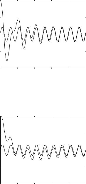
Fig. 4.7.1. Flow rate q(t) (solid curves) in an RLC system in series and in free dynamics, under conditions of overdamping, underdamping, and critical damping. Dashed line represents steady state flow rate.
|
1 |
|
|
|
|
|
flow rate q(t) |
0.5 |
|
|
|
|
|
0 |
|
|
|
|
|
|
normalized |
|
|
|
|
|
|
−0.5 |
|
|
|
|
|
|
|
−10 |
2 |
4 |
6 |
8 |
10 |
|
|
|
|
t / tL |
|
|
Fig. 4.7.2. Flow rate q(t) (solid curve) in an RLC system in series and in forced overdamped dynamics, with an oscillatory driving pressure drop. Dashed line represents steady state flow rate.
4.7 Transient and Steady States |
129 |
|
1 |
|
|
|
|
|
flow rate q(t) |
0.5 |
|
|
|
|
|
0 |
|
|
|
|
|
|
normalized |
|
|
|
|
|
|
−0.5 |
|
|
|
|
|
|
|
−10 |
2 |
4 |
6 |
8 |
10 |
|
|
|
|
t / tL |
|
|
Fig. 4.7.3. Flow rate q(t) (solid curve) in an RLC system in series and in forced underdamped dynamics, with an oscillatory driving pressure drop. Dashed line represents steady state flow rate.
|
1 |
|
|
|
|
|
flow rate q(t) |
0.5 |
|
|
|
|
|
0 |
|
|
|
|
|
|
normalized |
|
|
|
|
|
|
−0.5 |
|
|
|
|
|
|
|
−10 |
2 |
4 |
6 |
8 |
10 |
|
|
|
|
t / tL |
|
|
Fig. 4.7.4. Flow rate q(t) (solid curve) in an RLC system in series and in forced critically damped dynamics, with an oscillatory driving pressure drop. Dashed line represents steady state flow rate.

130 4 Forced Dynamics of the RLC System
the corresponding time is t/tL ≈ 5. To determine these times in seconds requires an estimate of the inertial time constant tL for the coronary circulation which, of course, is not known. Indeed, one of the main aims of lumped model studies is to determine such properties of the system.
Nevertheless, we may attempt to estimate tL by recalling from sections 2.4,5 (Eqs.2.4.5,2.5.5) that for flow in a single tube the resistance to flow and the inertial constant are given by
R = |
8μl |
(4.7.3) |
|
πa4 |
|||
|
|
||
L = |
4ρl |
(4.7.4) |
|
πd2 |
|||
|
|
where μ, ρ are respectively the viscosity and density of the fluid, and a, d are respectively the radius and diameter of the tube. From this, and from the definition of tL we then have
tL = |
L |
= |
ρa2 |
(4.7.5) |
|
|
|
seconds |
|||
R |
8μ |
||||
Taking ρ = 1.0 g/cm3 and μ = 0.04 g/(cm s), this becomes
tL = |
a2 |
(4.7.6) |
0.32 seconds |
where a is in centimeters.
Now, in a lumped model of the coronary circulation the characteristic parameters of the numerous tubes in the system are “lumped” together, which is equivalent to considering the system as a single tube that has these lumped properties. The problem, of course, is that these lumped properties are not known. Indeed, whether by theory or by experiment, the ultimate goal of lumped model studies is to determine not only the values of such properties but the legitimacy of the lumped parameter concept on which they are based.
Thus, from Eq. 4.7.6 we can only conclude that for a tube of 1cm radius, the equation gives a value of tL of approximately 3 seconds, while for a tube of 1mm radius, the corresponding value is 0.03 seconds. The transient state of an RLC system with these values of tL would then be approximately 15 tL in free dynamics and 5 tL in forced dynamics. The highest of these values is 45 seconds, the lowest is 0.15 seconds. Whether the true transient time of the coronary circulation lies within or indeed outside these estimates is not known. In the forced oscillatory dynamics of the coronary circulation tL would represent the time it takes the system to recover from a disturbance and return to steady state, thus knowing the actual value of this time constant would be of considerable clinical importance.

4.8 The Concept of Reactance |
131 |
4.8 The Concept of Reactance
The concepts of reactance and impedance arise in the dynamics of the RLC system in steady state. It is important to emphasize this point because these concepts are so widely used that it is usually only implied, but rarely stated, that their use is limited to steady state dynamics only, not to the transient state. Thus, in introducing these concepts here, and using them in subsequent sections, it must be clear from the outset that we are now dealing with only the particular solution of the governing equation (Eq. 3.2.5)
|
d2q |
+ |
dq |
1 |
q = |
1 d(Δp) |
|
|||
tL |
|
|
+ |
|
|
|
|
(4.8.1) |
||
dt2 |
dt |
tC |
R dt |
|||||||
and for this reason we no longer use the subscripts for the homogeneous and particular parts of the solution discussed in the previous section. It is implied here, and whenever these concepts are used, that q(t) now represents only the particular part of the solution, which, as discussed in the previous section, corresponds to the steady state dynamics of the RLC system.
Furthermore, a meaningful definition of reactance and impedance is only possible when Δp above, and consequently q(t), are simple oscillatory functions such as the trigonometric sine and cosine functions. We thus begin with the problem solved in Section 4.2, where the driving pressure drop is given by
Δp = Δp0 cos ωt |
(4.8.2) |
Steady state solution of Eq. 4.8.1 with this form of the pressure drop was obtained in Section 4.2 (Eq. 4.2.13), which we now write in the form
q(t) = Δp0 |
R cosR2 + S2 |
|
(4.8.3) |
|||
|
|
ωt + S sin ωt |
|
|
||
where |
|
|
|
|
|
|
|
1 |
|
|
(4.8.4) |
||
S = ωL − |
|
|
|
|||
ωC |
|
|||||
Using standard trigonometric identities, Eq. 4.8.3 can be simplified further to
q(t) = |
√ |
Δp0 |
|
cos(ωt − θ) |
(4.8.5) |
|
|
|
|||||
R2 + S2 |
||||||
where |
|
|
|
|
||
|
|
tan θ = |
|
S |
|
(4.8.6) |
|
|
R |
||||
|
|
|
|
|||
To discuss the nature and e ect of the quantity S now, we begin by noting that when S = 0, Eqs.4.8.5,6 give

132 4 Forced Dynamics of the RLC System
q(t) = |
Δp0 |
cos ωt |
(4.8.7) |
||
R |
|||||
|
|
|
|||
= |
Δp |
|
|
(4.8.8) |
|
R |
|
||||
|
|
|
|||
which we recognize as the simple expression for the flow rate through a resistance R when the driving pressure drop across it is Δp. Thus, in the dynamics of the RLC system the quantity S as defined in Eq. 4.8.4 embodies the combined e ects of inductance L and capacitance C such that when S = 0 the system behaves as a simple resistance R. When S = 0, it is clear from a comparison of Eq. 4.8.5 with Eq. 4.8.7 that S acts as an added form of resistance to flow, resulting from the presence of inductance and capacitance. It is also noted from the presence of ω in the expression for S that this form of resistance occurs only in oscillatory flow. By analogy with the same phenomenon in the flow of alternating current in an electric circuit, S is generally referred to as the “reactance”. It is a form of resistance to flow, but it di ers from R in that it only occurs in oscillatory flow. Also, unlike the viscous resistance R, the reactance S does not actually dissipate flow energy, it merely stores it and releases it within each oscillatory cycle [221].
From Eq. 4.8.4 we note that there are two ways in which the reactance S can be zero. First, when the capacitance and inductance e ects are simply absent, that is
L = 0 |
(4.8.9) |
||
1 |
= 0 |
(4.8.10) |
|
C |
|||
|
|
||
which together lead to S = 0. Second, when the values of ω, L, C are such that
C = |
1 |
(4.8.11) |
ω2L |
which again leads to S = 0. While the first of these circumstances is trivial, the second has clear physiological significance because it deals with the critical balance between the e ects of capacitance and inductance. To pursue this further, consider, in Eq. 4.8.4, that the frequency ω and inductance L are fixed so that the value of S now depends on the capacitance C only. It is convenient in this discussion to use the term “compliance” for the capacitance C. It is a more expressive term than “capacitance” because at higher values of the capacitance C a balloon is more elastic, more compliant, while at lower values of the capacitance C it is less elastic, less compliant.
Starting at the extreme where a balloon is rigid, compliance (C) is zero, and its reciprocal is infinite. The value of S from Eq. 4.8.4 is then infinite and negative, and the corresponding value of the phase angle θ from Eq. 4.8.6 is −π/2. Eq. 4.8.5 then indicates that the flow is leading the pressure drop by π/2. As the compliance gradually increases from this extreme value, the
4.8 The Concept of Reactance |
133 |
values of S and θ remain negative at first but continue to increase, until at some point they both become zero. The value of C at which this point is reached is given in Eq. 4.8.11, and we shall denote this value by C0, that is
C0 = |
1 |
(4.8.12) |
ω2L |
At this critical value of C the reactance is zero, the phase angle between the flow and pressure drop is zero, and the amplitude of the flow rate, which from Eq. 4.8.5 is given by
|q(t)| = |
√ |
Δp0 |
|
(4.8.13) |
||
|
|
|
|
|||
R2 + S2 |
|
|
|
|||
clearly has its highest value because S = 0. Thus, |
|
|||||
at C = C0 : |
S = 0 |
|
(4.8.14) |
|||
|
|
θ = 0 |
|
(4.8.15) |
||
|
|
|q(t)| = |
Δp0 |
(4.8.16) |
||
|
|
|
R |
|||
As compliance continues to increase beyond this point, the value of S becomes positive, the phase angle θ becomes positive, which means that flow is now lagging the pressure drop, and the amplitude of the flow rate begins to decrease again from its maximum value.
To illustrate these results graphically, it is convenient to use a normalized
form of the flow rate, namely |
|
|
|
|
|
||
|
|
(t) = |
q(t) |
|
(4.8.17) |
||
|
q |
|
|
|
|
||
|
Δp0/R |
|
|||||
= |
1 |
cos(ωt − θ) |
(4.8.18) |
||||
|
|
||||||
|
|
||||||
1 + (S/R)2 |
|||||||
Also, instead of using the actual capacitance C, it is more convenient to use the capacitive time constant
tC = CR |
(4.8.19) |
Since R is assumed to be constant, tC is a direct measure of C. Also, using the inertial time constant
tL = L/R |
(4.8.20) |
the reactance S can be expressed in terms of these time constants as
S |
= ωtL − |
1 |
(4.8.21) |
R |
ωtC |
134 4 Forced Dynamics of the RLC System
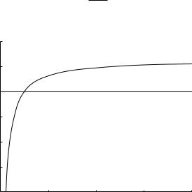
Fig. 4.8.1 shows the variation of the reactance as tC increases from zero (where capacitance and compliance are zero) to large values (where capacitance and compliance are large). In that sequence the value of S changes from large negative to positive, thus passing zero at one particular value of tC which we shall denote by tC0, and which from Eq. 4.8.12 is given by
tC0 = |
1 |
(4.8.22) |
ω2tL |
normalized reactance (S / R)
10 |
|
|
|
|
5 |
|
|
|
|
0 |
|
|
|
|
−5 |
|
|
|
|
−10 |
|
|
|
|
−15 |
|
|
|
|
−200 |
0.05 |
0.1 |
0.15 |
0.2 |
|
|
tC (seconds) |
|
|
Fig. 4.8.1. Normalized value of the reactance (S/R), as a function of the capacitive time constant tC . Of particular significance is the point at which reactance becomes zero, which occurs at tC = 1/4π2 ≈ 0.0253.
If the frequency of oscillation in cycles per second (Hz) is denoted by f , then the angular frequency ω is given by
ω = 2πf radians |
(4.8.23) |
As in previous sections, the inertial time constant tL may be used as the normalizing unit of time, which is equivalent to taking
|
tL = 1.0 seconds |
(4.8.24) |
|
With these values of ω and tL, Eq. 4.8.22 gives |
|
||
tC0 = |
1 |
≈ 0.0253 seconds |
(4.8.25) |
|
|||
(2π)2 |
|||
as seen in Fig. 4.8.1. At higher values of tC , as capacitance e ects become more significant, the normalized reactance S/R approaches the constant value, from
4.8 The Concept of Reactance |
135 |
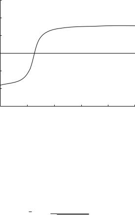
Eq. 4.8.21, 2π ≈ 6.283, again as seen in that figure. Corresponding values of the phase angle θ are shown in Fig. 4.8.2, where it is seen that the phase angle is zero at the same critical value of tC where the reactance is zero, namely at tC ≈ 0.0253. At higher values of tC (higher capacitance and compliance) the angle is positive, which means that flow is lagging behind the pressure drop, while at lower values of tC the reverse is true.
phase shift angle θ (degrees)
150 |
|
|
|
|
|
100 |
|
|
|
|
|
50 |
|
|
|
|
|
0 |
|
|
|
|
|
−50 |
|
|
|
|
|
−100 |
|
|
|
|
|
−1500 |
0.02 |
0.04 |
0.06 |
0.08 |
0.1 |
|
|
tC (seconds) |
|
|
|
Fig. 4.8.2. Phase angle θ between flow rate and pressure drop, as a function of the capacitive time constant tC . The angle becomes zero and changes sign at the same critical value of tC where reactance is zero (Fig. 4.8.1), namely tC = 1/4π2 ≈ 0.0253.
This change in phase shift is illustrated in Figs.4.8.3-5 where values of tC near the critical value are taken. It is remarkable that only a small departure from the critical value of tC is needed to produce a significant change in phase angle. A similar change occurs in the amplitude of the flow wave, which can be put in the normalized form
1 |
|
|q(t)| = 1 + (S/R)2 |
(4.8.26) |
In this form the amplitude has the normalized value of 1.0 when S = 0, which occurs at the critical value of tC . Figs.4.8.3-6 show clearly that this is the maximum value of the flow amplitude. At all other values of tC the flow wave is a ected both in phase and amplitude.
These results have remarkable implications regarding the phyiological system. While the RLC system in series does not appropriately model the coronary circulation (RLC in parallel will be considered in Chapter 6), it nevertheless points to the existence of conditions under which the system may
136 4 Forced Dynamics of the RLC System
|
1.5 |
|
|
|
|
|
1 |
|
|
|
|
q(t) |
|
|
|
|
|
flow rate |
0.5 |
|
|
|
|
0 |
|
|
|
|
|
normalized |
|
|
|
|
|
−0.5 |
|
|
|
|
|
|
|
|
|
|
|
|
−1 |
|
|
|
|
|
−1.50 |
0.5 |
1 |
1.5 |
2 |
|
|
|
t / tL |
|
|
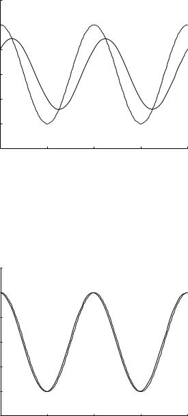
Fig. 4.8.3. Normalized flow rate (solid curve) compared with pressure drop (dashed curve) within the oscillatory cycle, and with tC = 0.03 seconds, which is just above critical value of tC = 0.0253 at which the two curves would be identical. Flow rate lags behind pressure drop and flow amplitude is below maximum.
|
1.5 |
|
|
|
|
|
1 |
|
|
|
|
q(t) |
|
|
|
|
|
flow rate |
0.5 |
|
|
|
|
0 |
|
|
|
|
|
normalized |
|
|
|
|
|
−0.5 |
|
|
|
|
|
|
|
|
|
|
|
|
−1 |
|
|
|
|
|
−1.50 |
0.5 |
1 |
1.5 |
2 |
|
|
|
t / tL |
|
|
Fig. 4.8.4. Normalized flow rate (solid curve) compared with pressure drop (dashed curve) within the oscillatory cycle, and with tC = 0.025 seconds, which is very close to critical value (at the critical value the two curves would be indistinguishable). Flow rate is in phase with pressure drop and flow amplitude is maximum.
4.9 The Concepts of Impedance, Complex Impedance |
137 |
|
1.5 |
|
|
|
|
|
1 |
|
|
|
|
q(t) |
|
|
|
|
|
flow rate |
0.5 |
|
|
|
|
0 |
|
|
|
|
|
normalized |
|
|
|
|
|
−0.5 |
|
|
|
|
|
|
|
|
|
|
|
|
−1 |
|
|
|
|
|
−1.50 |
0.5 |
1 |
1.5 |
2 |
|
|
|
t / tL |
|
|
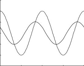
Fig. 4.8.5. Normalized flow rate (solid curve) compared with pressure drop (dashed curve) within the oscillatory cycle, and with tC = 0.02 seconds, which is just below critical value of tC = 0.0253 at which the two curves would be identical. Flow rate leads pressure drop and flow amplitude is below maximum.
operate most optimally, in the sense of minimizing the e ects of reactance. The mere existence of these conditions is clearly of significant clinical interest because it indicates that if the coronary circulation normally operates at or near a critical value of tC , then any change in the elasticity or other properties of the system, resulting from disease or clinical intervention, may move the system away from its optimal dynamics.
Furthermore, in the present system if tL is set equal to 1.0 seconds, which is not an unreasonable estimate following the discussion in Section 4.7, these favourable conditions occur at tC = 0.0253 seconds. While these two values may be inaccurate in absolute terms, they indicate that in relative terms the capacitive time constant may be two orders of magnitude smaller than the inertial time constant.
4.9 The Concepts of Impedance, Complex Impedance
The concept of “impedance”, like that of reactance, arises in the dynamics of the RLC system in steady state under a simple oscillatory driving pressure drop and, as emphasized in the previous section, it is only valid, indeed only meaningful, in that context. Again, the concept is borrowed from the flow of alternating current in electric circuits, but it has wide applications in the dynamics of the coronary circulation, specifically in the context of lumped models of the system.