The Physics of Coronory Blood Flow - M. Zamir

220 6 Composite Pressure-Flow Relations

the flow swings may be very large because they are free from the e ects of the resistor. In the coronary circulation, and in the cardiovascular system in general, capacitance is always in parallel with resistance because it is provided by the elasticity of the conducting vessels while resistance is provided by viscosity of the fluid, thus the flow always has the option of flowing through or inflating the vessels. The two options are in parallel. Any change in this property of the coronary system, which may be brought about, for example, by vasodilator drugs which cause the conducting vessels to fully inflate and thereby lose their ability to provide any further compliance, may disrupt the normal dynamics of the system because of the absence of normal capacitive e ects. Similarly, vascular spasm, whether it is induced by drugs or by regulatory mechanisms, will also alter the normal compliance of the system and thereby disrupt its normal dynamics.

The dynamics of the RLC system in series depend not only on the relative values of tC and tL but on their individual values too. The reason for this is that even when compliance is high, capacitive e ects cannot dominate the flow because they are still constrained by any remaining inertial e ects in the system. Only when the latter are reduced to an insignificant level do capacitance e ects dominate. While in the coronary circulation, as stated previously, capacitance e ects are always in parallel, the RLC system in series provides an important “ground state” reference for parallel and hybrid lumped models.

Capacitive e ects are much more pronounced when capacitance is in parallel with other elements of the RLC system. This is important because capacitive e ects in the coronary circulation are in fact in parallel, as they are caused by elasticity of the conducting vessels. Therefore, coronary flow has the (parallel) option of flowing through or inflating the vessels. Thus, again, a change in the capacitive property of the coronary arteries, by drugs, spasm, or disease can drastically change the character of the flow wave.

7

Lumped Models

7.1 Introduction

A succession of lumped models, guided by a series of observations and sometimes heroic experiments, have been the principal means by which an understanding of the dynamics of the coronary circulation has evolved

or material errors. The following sampling, in chronological order, provides some sign posts which will lead the keen reader to many more references: [85, 86, 83, 169, 19, 22, 111, 49, 59, 65, 128, 40, 121, 32, 110, 102, 157, 24, 33, 130, 195, 29, 107, 90, 115, 97, 98, 183, 131, 162, 163, 47].

The early notion of the coronary circulation as a “windkessel”, a combination of resistance and capacitance, was a natural o -shoot from the dynamics of the systemic circulation as it was understood at the time [135, 141, 153], but the special characteristics of the coronary circulation soon became apparent [83]. The mechanically hostile milieu in which coronary vasculature is embedded, the peculiar and mostly diastolic coronary flow wave, the high coronary flow reserve, and the severe and multifaceted regulatory environment in which the coronary circulation operates were special issues that had to be dealt with. While some progress has been made in each case, essentially the same issues remain outstanding today. Whether because a certain characteristic cannot be accurately modelled or because it can be modelled in more than one way, an all-encompassing model, lumped or otherwise, able to deal with these issues as they combine in the dynamics of the coronary circulation is yet to emerge. The subject remains very much a “work-in-progress”.

Most lumped models of the coronary circulation to date have been based on essentially three types of elements, namely the elements of the RLC system. However, the total number of elements used in a given model, the number of each type, and the number of di erent ways in which these can be arranged have provided the scope for a wide range of di erent models. The purpose of

222 7 Lumped Models

this chapter is not to enumerate these models but to return to the foundations on which they stand. We return to the basic elements of the RLC system and proceed from there in a systematic manner to examine the way in which they may give rise to some of the characteristic features observed in the dynamics of the coronary circulation. The intention here is to provide not complete models but the conceptual ingredients from which such models would be constructed.

As we have seen in earlier chapters, in the RLC system the resistance R is taken to represent the viscous resistance between the moving fluid and the vessel wall, the inductance L to represent the inertia of the moving fluid, and the capacitance C the elasticity of the vessel wall. These three e ects provide an appropriate starting point because it is known on purely physical grounds that these e ects do exist in the coronary circulation and must therefore play a role in its dynamics. Of course, other e ects exist too: viscoelasticity within the vessel wall, intramyocardial pressure surrounding coronary vessels, wave reflections within the coronary vascular tree, and myogenic vasomotor activity and other control mechanisms, but these are all seen to exist at a higher level of complexity. Models of the coronary circulation presented in the past have been mostly at this higher level. In this chapter we focus on the foundations on which these models are based.

Specifically, we examine four di erent arrangements of the RLC elements which deal with di erent dynamical issues in somewhat increasing degree of complexity. In a sense they are basic lumped models which may be referred to as LM 0, LM 1, LM 2, LM 3. As a shorthand notation we present the elements of the model inside curly brackets, with a comma representing a parallel connection between two elements and a plus sign representing a series connection. In this notation the four models are given by:

The models are examined in more detail below. In particular, pressure-flow relations under these models are examined, using the cardiac pressure wave as the driving pressure.

7.2 LM0: {R,C}

The simplest lumped model of the coronary circulation, which we shall refer to as LM 0, is the so-called “windkessel” model, which was first devised for the cardiovascular system as a whole [135, 141, 153]. In that context, it was recognized early that the cardiac pressure pulse generated by the left ventricle is not transmitted directly to the periphery but is first absorbed by the compliance of the aorta and its major branches. It is as if the energy of the

pulse is first expended on inflating a balloon, and then as the pulse abates, the balloon deflates and returns this energy to drive the flow downstream somewhat more gently than the original pulse. The same scenario is believed to occur in the coronary circulation.

Since the two main coronary arteries that bring blood supply into the coronary circulation have their origin at the base of the ascending aorta just as it leaves the left ventricle (Figs. 1.3.1, 2), flow entering these arteries is subject to the full force of the cardiac pressure pulse. And it is well established that the main coronary arteries have a considerable degree of compliance, which can in fact be easily observed in the course of coronary cine-angiography. Thus, the ingredients for a windkessel scenario, namely a pulsating pressure and compliant vessels, are present in the coronary circulation as they are in the cardiovascular system as a whole. Indeed, compliance, or capacitance e ects, within the coronary circulation are believed to be the result of not only the elasticity of the coronary vessels but also the enormous contraction and relaxation of the cardiac muscle tissue in which many of the coronary vessels are embedded. Thus, capacitance e ects rank high in the dynamics of the coronary circulation.

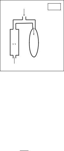
As discussed at great length in Chapter 2, capacitance e ects in the coronary circulation and in the cardiovascular system as a whole do not occur in isolation but in combination with the ever-present resistance to flow due to viscous e ects between moving blood and the vessel wall. If flow in the coronary circulation were steady, the most elementary model of the circulation would consist of only a driving pressure and the e ect of that resistance, as discussed in Section 2.4. But because of the pulsatile nature of the driving pressure, the most elementary model of the coronary circulation must take into account the e ects of capacitance, and thus include both capacitance and resistance. Furthermore, the nature of capacitance e ects in the coronary circulation is such that flow has the option of moving against the resistance or capacitance, that is, the option of moving forward or inflating the vessels. In other words, the e ects of capacitance and resistance are in parallel. In the context of previous sections, therefore, the most elementary model of the coronary circulation is RC in parallel, as shown in Fig. 7.2.1.

The complex impedance for RC in parallel was found in Section 4.9, Eqs.4.9.34,35, namely

where ω is the angular frequency of oscillation of the driving pressure. For a composite pressure wave consisting of N harmonics the impedance will be

224 7 Lumped Models

LM0

qtot

R qcap C

qres

Fig. 7.2.1. The most elementary model of the coronary circulation is a resistance R and capacitance C in parallel, originally known as the “windkessel” model, and which we shall refer to as LM 0 : {R,C}.

di erent for each harmonic because of their di erent frequencies and, as before, we shall use the notation

where n denotes a particular harmonic and ωn is the angular frequency of that harmonic.

Following the same steps as in Chapter 6, and omitting some of the details, we find the harmonics of the oscillatory flow wave as

where pn(t) are the harmonics of the driving pressure in their complex exponential form, namely

n = 1, 2, . . . , N

226 7 Lumped Models

The individual parallel flow waves are obtained by adding the harmonics of each flow, that is

R × qr,res(t) = R × q1r,res + R × q2r,res + . . . + R × qN r,res (7.2.20)

R × qr,cap(t) = R × q1r,cap + R × q2r,cap + . . . + R × qN r,cap (7.2.21)

As before, only the oscillatory parts of the pressure and flow waves are shown, the steady parts being omitted to make the graphical comparison of these waves easier by using the same scale.

Results, comparing total and individual R-scaled flow waves, using the cardiac pressure wave and a relatively low value of the capacitive time constant, namely tC = 0.01 s, are shown in Fig. 7.2.2. At this value of tC , which corresponds to low compliance (the balloon is sti ), capacitive flow is small. Resistive flow, which is independent of capacitive e ects because of the parallel arrangement, is identical in form with the pressure waveform on an R- scaled basis and is thus represented by the same curve as the pressure wave in Fig. 7.2.2. Total flow, again on an R-scaled basis, is only slightly di erent in form from the pressure waveform, the di erence being due to the small capacitive flow.

Fig. 7.2.2. Pressure-flow relations under LM 0, with a relatively low value of the capacitive time constant, namely tC = 0.01 s. Heavy solid curve (p, res) represents both the pressure wave and the R-scaled resistive flow, which are identical because the resistance is in parallel. Thin solid curve (tot) represents total flow into the parallel system, and the dashed curve (cap) represents capacitive flow. Total flow is dominated by resistive flow and is only slightly a ected by capacitance.

Fig. 7.2.3. Pressure-flow relations under LM 0 as in Fig. 7.2.2, but here with a considerably higher value of the capacitive time constant, namely tC = 0.2 s. Total flow (tot) is now dominated by capacitive e ects and follows the curve of capacitive flow (cap).

At a higher value of the capacitive time constant, namely tC = 0.2 s, the situation is drastically changed as seen in Fig. 7.2.3. Here compliance is considerably higher (the balloon is more elastic), allowing correspondingly higher capacitive flow. The form of the R-scaled total flow wave is considerably di erent from that of the pressure wave because total flow is dominated by capacitive flow. Resistive flow is the same as in Fig. 7.2.2, but here, because of much higher capacitive flow, resistive flow is a relatively less significant part of total flow.

It is important to recall that capacitive flow is driven not by a pressure di erence but by the rate of change of a pressure di erence, as discussed at great length in Section 2.6. In present notation, where p(t) actually represents a pressure di erence, this means that capacitive flow depends not on p(t) but

This equation indicates clearly that R-scaled capacitive flow is in fact proportional to the slope of the pressure curves in Figs. 7.2.2, 3, the constant of

7.3 LM1: {R1,{R2+C}} 229

proportionality being the capacitive time constant tC . Thus, if we compare the R-scaled capacitive flow, R × qcap(t) not with the pressure curve but with its slope, we expect agreement between the two. This comparison is shown in Figs. 7.2.4, 5.

7.3 LM1: {R1,{R2+C}}

It is clear from results of the previous section that capacitive e ects in the coronary circulation are not likely to be present in isolation, or in pure form, because this would lead to large swings in the flow waveform which are not observed in the physiological system. This has led to the view that the compliance of blood vessels, which is responsible for capacitance e ects, is produced by viscoelasticity rather than pure elasticity of the vessel wall [79, 204, 78, 52, 55, 4]. Thus, capacitive flow, the filling of the balloon, is resisted not only by the elasticity of the vessel wall but also by some viscoelastic forces within the wall.

We recall from Section 2.6 that in the case of purely elastic capacitance the relation between the pressure p(t) inside a balloon and the rate of flow q(t) into it is such that the flow rate depends on the rate of change of pressure, dp/dt, rather than on the pressure itself. We refrain from calling this a “pressure gradient” because it is a rate of change of pressure with time, not to be confused with a rate of change of pressure along a tube. The relation is such that

where C is the capacitance constant. The flow rate (into the balloon) and the rate of change of pressure have the same sign, so that when the rate of change of pressure is positive (pressure is increasing), flow rate into the balloon is positive, and vice versa. When the rate of change of pressure is zero, capacitive flow, flow into or out of the balloon, is zero.

When the balloon wall is not purely elastic but has some viscoelastic component, the relation between pressure and flow is of the form

where B is a constant relating to the viscoelastic property of the wall. Here the rate of change of pressure required to maintain flow into or out of the balloon depends not only on the flow rate but on the rate of change of flow rate. The consequence of this in modelling the coronary circulation is that it changes the complex impedance for a capacitive element.

We recall from Section 4.9 that the complex impedance for a purely elastic capacitor is given by (Eq. 4.9.36)