

The Physics of Coronory Blood Flow - M. Zamir
.pdf270 8 Elements of Unlumped-Model Analysis
streamwise distance X (normalized)
|
00 |
0.5 |
1 |
1.5 |
2 |
P(X) |
-0.5 |
|
P0 |
|
|
|
|
|
|
|
|
pressure |
-1 |
|
|
|
|
|
|
|
|
P2 |
|
-1.5 |
|
|
|
|
|
nondimensional |
|
|
|
|
|
|
|
|
|
P1 |
|
-2 |
P0 |
|
|
|
|
|
|
|
|
||
-2.5 |
|
P2 |
|
|
|
|
P1 |
|
|
||
|
|
|
|
|
|
|
-3 |
|
q a4 |
|
|
Fig. 8.4.3. Pressure distributions within the three vessel segments forming an arterial bifurcation, under the idealized conditions of steady Poiseuille flow and on the assumption of a power law relation between the radius of each vessel and the flow rate through it. If the power law index is more than 3, as it is here, the pressure drop in the branch with the smaller radius (branch-2) is lower than that in the other branch.
where r is radial coordinate within the vessel and a is its radius. Using the results for flow in a tube and resistance to flow in sections 2.3,4, this equation for the shear stress can be expressed in terms of the flow rate, to give
τw = |
4μ |
|
q |
|
(8.4.32) |
|
π |
|
a3 |
||||
or in terms of the pressure drop, to give
τw = − |
Δp |
|
a |
|
(8.4.33) |
|
2μ |
l |
|
||||
The first of these results indicates that if a power law relation as in Eq. 8.4.22 exists between the radius of a vessel and the flow rate which it carries, then the shear stress in vessels of di erent radii varies as
τw aγ−3 |
(8.4.34) |
If the value of γ is less than 3, the shear stress will be higher in vessels of smaller radii, which clearly cannot be supported on physiological grounds. If the value of γ is more than 3, the shear stress will be lower in vessels of smaller

8.4 Steady Flow Through a Bifurcation |
271 |
streamwise distance X (normalized)
|
00 |
0.5 |
1 |
1.5 |
2 |
P(X) |
-0.5 |
P0 |
|
|
|
|
|
|
|
|
|
pressure |
-1 |
|
|
|
|
-1.5 |
|
|
P2 |
|
|
nondimensional |
|
|
|
||
|
|
|
P1 |
|
|
-2 |
|
|
|
|
|
|
P0 |
|
|
|
|
-2.5 |
|
|
|
|
|
|
P2 |
|
|
|
|
|
|
|
|
|
|
|
|
P1 |
|
|
|
|
-3 |
q a3 |
|
|
|
|
|
|
|
|
Fig. 8.4.4. Pressure distributions within the three vessel segments forming an arterial bifurcation, under the idealized conditions of steady Poiseuille flow and on the assumption of a power law relation between the radius of each vessel and the flow rate through it. If the power law index is equal to 3, as it is here, the pressure drop is the same along both branches.
radii, which is more plausible on physiological grounds. But if the value of γ is equal to 3, the shear stress in Eq. 8.4.32 will be altogether independent of the radius a, which means that the shear stress will be the same in vessels of di erent radii. With this value of γ, the flow rate is proportional to the third power of the radius, or conversely, the radius is proportional to the cube root of the flow rate. This relation between the radius and flow rate is widely known as the “cube law” and is of particular interest because it was first derived by showing that it actually provides an optimum compromise between the pumping power required to drive the flow through the bifurcation, which is lower when the vessel radii are large, and the metabolic power required to maintain the volume of blood contained within the three vessels forming the bifucation, which is lower when the vessel radii are small [147, 212, 213].
Of interest in the present context is the second of the above results, namely that in Eq. 8.4.33, which indicates that if the length of a vessel is assumed to be proportional to its radius then the pressure drop becomes proportional to the shear stress, and hence everything that has been said above about the shear stress now applies equally to the pressure drop. In particular, for the two branches at a bifurcation, if the value of γ is more than 3, the pressure drop along the branch with the smaller radius is lower than that along the

272 8 Elements of Unlumped-Model Analysis
branch with the larger radius. This is somewhat unlikely on physiological or fluid dynamic grounds. On the other hand, if the value of γ is less than 3, the reverse is true, which is more plausible on both grounds. If the value of γ is equal to 3, the pressure drop is the same along both branches. These results are shown in Figs. 8.4.2–4.
The interesting conclusion from this discussion is that from the point of view of the shear stress acting on endothelial tissue, the more likely values of γ are 3 or higher, but from the point of view of pressure drop the more likely values are 3 or lower. The only possible compromise between these two conflicting requirements is clearly γ = 3, and this lends further theoretical support to the cube law. As stated earlier, values of γ based on actual measurements from the cardiovascular system have shown much scatter not only within the range of 2−4 but also outside this range [220]. The scatter, however, is generally found to center around the value γ = 3.
8.5 Pulsatile Flow in a Rigid Tube
We have seen in Sections 2.3 and 8.3 that in steady flow through a tube the pressure varies linearly along the tube, dropping from a high at entrance to a low at exit, the di erence between the two being the pressure drop driving the flow. All other properties of the flow field such as the flow rate, the shear stress at the tube wall, or velocity at any point within the tube are constant in the sense that they do not depend on the streamwise coordinate x. Only the pressure varies along the tube, but the pressure drop between the two ends of the tube is constant. These features of the flow are embodied by the equation for Poiseuille flow presented in Section 2.3 which we reproduce here using a subscript s to indicate that the flow properties are for steady flow only, as distinct from flow properties in pulsatile flow which we consider below. Thus, from Eq. 2.3.1 we write
us(r) = |
ks |
(r2 − a2) |
(8.5.1) |
4μ |
where us is the streamwise velocity within the tube, μ is viscosity of the fluid, a is the tube radius, r is radial coordinate measured from the tube axis, and ks is pressure gradient defined by (Eq. 2.3.2)
ks = |
Δps |
(8.5.2) |
|
l |
|||
|
|
where l is the length of the tube and Δps is the pressure di erence between the two ends of the tube.
It must be emphasized that the reference here is to fully developed flow in a tube as described in Section 2.3. While in practice flow in a tube is rarely fully developed along its full length, we continue to make this assumption here

8.5 Pulsatile Flow in a Rigid Tube |
273 |
as in the previous three sections because it is necessary in the analysis of flow in a large number of tubes, as in a vascular tree.
Under the assumption of fully developed flow, when the pressure drop between the two ends of a rigid tube is not constant but varies in time, flow properties within the tube vary in time too but, again, they do not vary along the tube. In other words, when the driving pressure drop is a function of time, flow properties within the tube become functions of time too but not functions of the streamwise coordinate x. As the pressure drop changes from one point in time to the next, flow properties change in the same way at every point along the tube. This singular behaviour is only possible when (a) the tube is rigid and (b) the fluid is incompressible; both of these conditions are assumed to prevail in this section.
Of particular interest in this section is flow in a tube when the driving pressure drop Δp is a periodic function of time, which may be a simple sinusoidal wave or a composite wave as discussed in Chapter 5. A periodic pressure drop along a tube may be thought to arise from a fixed pressure at the downstream end of the tube and a periodic pressure at the upstream or “input” end. For this reason we often refer to a periodic pressure drop as the “input pressure wave”.
If the input pressure waveform has a nonzero mean, as discussed in Section 5.6 (Fig. 5.6.1), then that mean value will serve as a constant pressure drop, producing steady Poiseuille flow within the tube, while the remaining part of the pressure will be purely oscillatory. Denoting the constant part of the waveform by Δps, as in Section 5.2, and the oscillatory part by Δpφ, we may then write
Δp(t) = Δps + Δpφ(t) |
(8.5.3) |
||||
or, in terms of pressure gradients, as in Eq. 8.5.2, |
|
||||
k(t) = ks + kφ(t) |
(8.5.4) |
||||
where |
|
|
|
|
|
k(t) = |
Δp(t) |
(8.5.5) |
|||
l |
|
||||
|
|
||||
kφ(t) = |
Δpφ(t) |
(8.5.6) |
|||
l |
|
||||
|
|
||||
By definition, Δps is the average value of Δp(t) over one oscillatory period T as discussed in Section 5.2, Eq. 5.2.15, that is
|
1 |
0 |
T |
|
|
Δps = |
Δp(t)dt |
(8.5.7) |
|||
T |
and, as a consequence, the purely oscillatory part of the waveform has a zero average over one oscillatory period, that is

274 |
8 Elements of Unlumped-Model Analysis |
|
|
T |
|
|
Δpφ(t)dt = 0 |
(8.5.8) |
0
Because the equations governing fully developed flow in a tube are linear, these two parts of the driving pressure can be dealt with separately, each producing a flow field as if it were the only driving pressure, and the two resulting flow fields are then added to produce the complete flow field. The situation is precisely the same as that in which the harmonic components of a composite pressure wave and the flows which they produce can be treated separately and the results are then added, as discussed in Section 6.2. Indeed, here too, the oscillatory part of the pressure, pφ(t), may itself be a composite wave which is then decomposed into harmonic components that are dealt with as in Chapter 6.
As a matter of terminology, when Δp(t) is a periodic function of time we shall refer to the flow which it produces as “pulsatile flow”, to the flow which Δps produces as “steady flow”, and to the flow which Δpφ(t) produces as “oscillatory flow”. Because the steady and the oscillatory parts of pulsatile flow can be dealt with separately as discussed above, and because steady flow in a tube has already been dealt with in Section 2.3, it remains to deal with only the oscillatory part of the flow.
A classical solution of the equations governing oscillatory flow in a rigid tube exists for an oscillatory pressure gradient of the form
kφ(t) = k0eiωt |
(8.5.9) |
= k0(cos ωt + i sin ωt) |
(8.5.10) |
In other words, the driving pressure consists of a simple sine or cosine wave with amplitude k0. We recall that, in this complex exponential formulation, the solution obtained is also in complex form where the real part describes the flow when the driving pressure is of the form k0 cos ωt, and the imaginary part describes the flow when the driving pressure is of the form k0 sin ωt.
For the oscillatory flow velocity field within the tube, the solution gives [177, 208, 194, 221]
uφ(r, t) = |
ik0a2 |
1 − |
J0(ζ) |
eiωt |
(8.5.11) |
μΩ2 |
J0(Λ) |
where J0 is Bessel function of order zero of the first kind, and
Ω = |
|
μ |
|
|
a |
(8.5.12) |
||||
|
|
|
ρω |
|
|
|
|
|||
|
|
|
|
|
|
|
|
|
|
|
Λ = |
i√− |
1 |
Ω |
(8.5.13) |
||||||
2 |
|
|||||||||
ζ(r) = |
Λ |
r |
|
|
(8.5.14) |
|||||
|
|
|||||||||
a |
|
|||||||||

8.5 Pulsatile Flow in a Rigid Tube |
275 |
To interpret uφ(r, t) in relation to the corresponding Poiseuille flow velocity in steady flow, namely us(r), it is convenient to use as a reference the maximum velocity in Poiseuille flow (Eq. 8.5.1) which occurs on the axis of the tube (r = 0), namely
uˆs = us(0) |
(8.5.15) |
||
= |
−ksa2 |
(8.5.16) |
|
4μ |
|||
|
|
||
Also, comparison between the steady and the oscillatory velocity profiles is made easier by taking the amplitude of the oscillatory pressure gradient to be the same as the pressure gradient in steady flow, that is, we take
k0 = ks |
(8.5.17) |
Nondimensional forms of the steady and the oscillatory velocity profiles are then defined by (Eq. 8.5.1)
us(r) |
= 1 − |
r2 |
(8.5.18) |
|
uˆs |
|
a2 |
||
uφ(r, t) |
= |
4 |
1 − |
J0(ζ) |
eiωt |
(8.5.19) |
uˆs |
iΩ2 |
J0(Λ) |
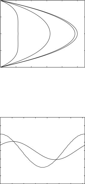
Evaluation of the last expression requires values of the Bessel functions, which are available numerically in math tables and in most computational programs [137, 198]. Because both us(r) and uφ(r, t) have been normalized in the same way, they can be compared graphically on the same scale, as shown in Fig. 8.5.1. The figure compares the oscillatory velocity profile with the corresponding profile in Poiseuille flow at di erent times within the oscillatory cycle. The comparison is made when the oscillatory flow is driven by the real part of the oscillatory pressure gradient, namely k0 cos ωt (k0 = ks). Thus, at t = 0 the oscillatory flow and the Poisuille flow are momentarily driven by the same pressure gradient and, in the absence of other factors, we would expect the two velocity profiles to be the same at that point in time within the oscillatory cycle.
The failure of peak velocity in oscillatory flow to reach the same value as peak velocity in Poiseuille flow (normalized at 1.0), is due clearly to inertial e ects. More accurately the di erence between the two is a function of the nondimensional frequency parameter Ω as defined in Eq. 8.5.12, also known as the Womersley number, which combines the e ects of frequency of oscillation, tube radius, and both the density and viscosity of the fluid. The di erences observed in Fig. 8.5.1 occur with Ω = 2.0. In particular, the velocity profiles at peak pressure gradient, which occurs at ωt = 0, is short of maximum Poiseuille flow velocity at this value of Ω. Results at higher and lower values of Ω are shown in Fig. 8.5.2.

276 8 Elements of Unlumped-Model Analysis
(normalized) |
1 |
|
|
|
|
|
|
|
|
|
|
|
|
||
0.5 |
|
|
|
|
|
|
|
|
|
|
|
|
|
|
|
distance |
0 |
|
250 |
300 |
100 |
0 |
40 |
|
|
||||||
radial |
−0.5 |
|
|
|
|
|
|
|
|
|
|
|
|
|
|
|
−1 |
|
|
|
|
|
|
|
−1 |
−0.5 |
0 |
0.5 |
|
1 |
|
|
|
|
|
normalized velocity |
|
|
|
Fig. 8.5.1. Velocity profiles of oscillatory flow in a rigid tube, driven by a pressure gradient of the form ks cos ωt where ks is a constant, ω is frequency and t is time. The profiles are shown at di erent times within the oscillatory cycle, as indicated by the value of the phase angle ωt (in degrees) on each curve. For comparison, the bold curve represents the velocity profile in Poiseuille flow driven by a pressure gradient ks. Velocities are normalized so that their values are comparable on the same scale. The di erences between the oscillatory profiles at di erent points in time within the oscillatory cycle and the Poiseuille flow profile indicate that peak velocity in oscillatory flow is lower than that in Poiseuille flow and occurs at a later time than peak pressure gradient, which occurs at ωt = 0.
Oscillatory flow rate qφ(t) is given by |
|
|
|
|||
qφ(t) = 0a |
2πruφ(r, t)dr |
|
(8.5.20) |
|||
= |
iπksa4 |
1 − |
2J1(Λ) |
eiωt |
(8.5.21) |
|
μΩ2 |
ΛJ0(Λ) |
|||||
and normalizing in terms of the corresponding flow rate in Poiseuille flow
qs = |
0a |
2πrus(r)dr |
(8.5.22) |
|
= |
|
−ksa2 |
(8.5.23) |
|
|
8μ |
|||
|
|
|
||
we have
qφ(t) |
= |
8 |
1 − |
2J1(Λ) |
eiωt |
(8.5.24) |
qs |
iΩ2 |
ΛJ0(Λ) |
radial distance (normalized)
1
0.5
0
−0.5
−10
8.5 Pulsatile Flow in a Rigid Tube |
277 |
3 |
2 |
1 |
0.2 |
0.4 |
0.6 |
0.8 |
1 |
|
normalized velocity |
|
|
|
Fig. 8.5.2. Velocity profiles at peak pressure gradient ks cos ωt, which occurs at ωt = 0, and di erent values of the nondimensional frequency parameter Ω as indicated on individual curves. The bold curve represents the velocity profile in Poiseuille flow driven by a pressure gradient ks.
|
2 |
|
|
|
|
|
|
|
rate (normalized) |
1.5 |
|
|
|
|
|
|
|
1 |
|
|
|
|
|
|
|
|
0.5 |
|
|
|
|
|
|
|
|
0 |
|
|
|
|
|
|
|
|
flow |
−0.5 |
|
|
|
|
|
|
|
oscillatory |
|
|
|
|
|
|
|
|
−1 |
|
|
|
|
|
|
|
|
−1.5 |
|
|
|
|
|
|
|
|
|
|
|
|
|
|
|
|
|
|
−20 |
50 |
100 |
150 |
200 |
250 |
300 |
350 |
|
|
|
phase angle (degrees) |
|
|
|||
Fig. 8.5.3. Oscillatory flow rate qφ(t) (solid) compared with the driving pressure gradient kφ(t) (dashed) for flow in a rigid tube with frequency parameter Ω = 3.0. Flow rate lags behind the pressure gradient and peak flow is significantly lower than the corresponding normalized Poiseuille flow value of 1.0.
278 8 Elements of Unlumped-Model Analysis
|
amplitude |
1.5 |
|
|
|
|
|
|
|
|
|
|
|
|
|
|
|
||
|
0.5 |
|
|
|
|
|
|
|
|
|
|
1 |
|
|
|
|
|
|
|
|
|
0 |
|
|
|
|
|
|
|
|
|
|
|
|
|
|
|
|
|
phase |
|
50 |
|
|
|
|
|
|
|
|
|
|
|
|
|
|
|
||
|
0 |
|
|
|
|
|
|
|
|
flow |
|
|
|
|
|
|
|
|
|
|
|
|
|
|
|
|
|
|
|
oscillatory |
|
−50 |
|
|
|
|
|
|
|
|
|
|
|
|
|
|
|
|
|
|
−1000 |
|
|
|
|
|
|
||
|
2 |
4 |
6 |
8 |
10 |
||||
|
|
|
|
|
frequency parameter Ω |
|
|
|
|
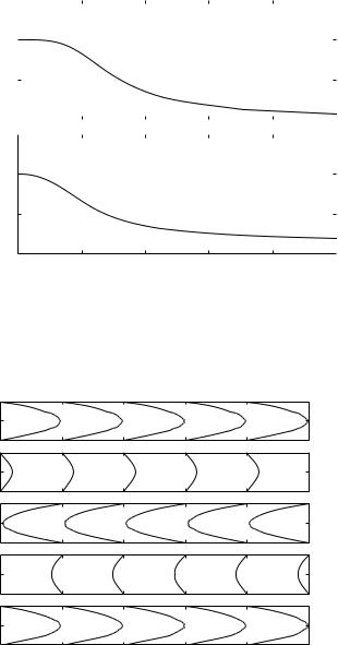
Fig. 8.5.4. Amplitude and phase of oscillatory flow rate qφ(t) at di erent values of the frequency parameter Ω.
radial distance (normalized) |
|
|
|
|
|
1 |
|
|
|
|
|
0 |
|
|
|
|
|
−10 |
1/0 |
1/0 |
1/0 |
1/0 |
1 |
|
|
axial velocity (normalized) |
|
|
|
0
90
180
270
360
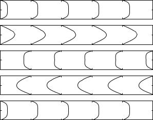
Fig. 8.5.5. Velocity profiles in pulsatile flow in a rigid tube at di erent times within the oscillatory cycle, indicated in degrees on the right of each panel, and with frequency parameter Ω = 1.0. A characteristic of pulsatile flow in a rigid tube is the absence of any change in the velocity profile as the flow progresses along the tube. The fluid moves in tandem at all positions along the tube.
8.6 Pulsatile Flow in an Elastic Tube |
279 |
radial distance (normalized)
1
0
−1
0
90
180
270
360
0 |
1/0 |
1/0 |
1/0 |
1/0 |
1 |
|
|
axial velocity (normalized) |
|
|
|
Fig. 8.5.6. Velocity profiles in pulsatile flow in a rigid tube at di erent times within the oscillatory cycle as in Fig. 8.5.5 but here with the frequency parameter Ω = 3.0.
Variation of the flow rate within the oscillatory cycle, with Ω = 3.0, is shown in Fig. 8.5.3. At this value of Ω peak flow rate is significantly lower than the normalized Poiseuille flow value of 1.0, and it lags behind the driving pressure gradient. At higher values of Ω peak flow diminishes further and the phase lag increases, as shown in Fig. 8.5.4.
One of the characteristics of pulsatile flow in a rigid tube is the absence of any change in the flow field as the flow progresses along the tube. The fluid moves in tandem at all positions along the tube, as shown in Figs. 8.5.5, 6, in other words the flow field is entirely independent of the streamwise coordinate x along the tube. This type of flow is only possible when the tube is strictly rigid. We shall see later that in the presence of any elasticity within the tube wall, pulsatile flow within the tube becomes a propagating wave and the flow field becomes a function of the streamwise coordinate x.
8.6 Pulsatile Flow in an Elastic Tube
A key di erence between flow in a rigid tube and that in an elastic tube is that in a rigid tube a local change in pressure is “sensed” instantaneously all along the tube, while in an elastic tube a local change in pressure is first absorbed locally by the elasticity of the tube wall and only then transmitted to other regions of the tube as illustrated schematically in Fig. 8.6.1. In particular, when the input pressure driving the flow in a rigid tube rises and falls in an oscillatory manner, as we saw in Section 8.5, the rise and fall in pressure has its