The Physics of Coronory Blood Flow - M. Zamir

300 9 Basic Unlumped Models

The challenge for unlumped model analysis of the coronary circulation is to (1) extract salient features of the coronary network that are more global in nature, such as the scale of the network, its general branching structure, and the flow rate that it is required to carry compared with that in the systemic circulation and to use combinations and variations of such features to demonstrate the type of dynamics that they can or cannot produce; (2) show how the propagating pressure wave driving the flow is likely to evolve under di erent models and properties of the coronary arterial tree and under di erent circumstances; and (3) determine under what circumstances wave reflections are likely to a ect the flow and therefore to what extent they may play a significant role in the dynamics of the coronary circulation. These issues are considered in the present chapter.

9.2 Steady Flow in Branching Tubes

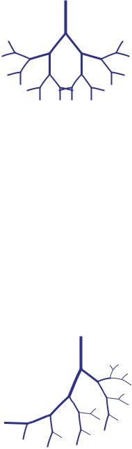
Arterial trees are generally found to consist of a succession of bifurcations whereby a root vessel segment divides into two branches, then each of the branches in turn divides into two branches, etc. [212]. The “symmetry” of each bifurcation, that is the relative radii of the two branches, is measured by the bifurcation index α = a2/a1 introduced in the previous section, where a1, a2 are radii of the two branches, subscript 1 being reserved by convention to the branch with the larger radius. The branching process is illustrated schematically in Fig. 9.2.1 where α = 1.0 and in Fig. 9.2.2 where α = 0.7. In each case, the value of α is the same at every bifurcation within the tree structure, thus producing a degree of uniformity which is not characteristic of arterial trees in the cardiovascular system where it is found that the value of α varies widely throughout the tree [224, 215, 226, 106, 218, 220]. Nevertheless, these theoretical structures are useful for the purpose of the present section, which is to analyse the pressure distribution in steady flow along such a vascular tree structure by generalizing the results of the previous chapter.

The strategy we follow is based on that used for a single bifurcation in the previous chapter. Here too the pressure distribution within the tree structure is determined simply by following all possible paths from the root segment of the tree to the terminal branch segments. Since each of these paths is unique and consists of a simple succession of tube segments in series, the results of Section 8.3 for tubes in series can then be used, noting only that the flow rate in this succession of tube segments is not the same but varies according to the bifurcation rules discussed in the previous chapter.

To carry out this strategy, the notation of the previous chapter must clearly be generalized to cater for a much larger number of branches. The term “branches” used in the previous chapter to identify the two branch vessel segments at a bifurcation is no longer adequate here because most vessel segments within the tree structure are both parents and branches. The only vessel segments that can be identified by name here are the root segment and

302 9 Basic Unlumped Models

j+1,2k-1 j+1,2k

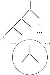
Fig. 9.2.3. A notation scheme for identifying the position of vessel segments in a branching tree structure. Each segment is assigned a coordinate pair j, k in which the first identifies the level of the tree at which the segment is located, and the second identifies the sequential position of that segment among other segments at that level of the tree. The insert shows that in general at each bifurcation one of the two branch segments has an odd sequential number and the other has an even sequential number. We use the convention of reserving the odd sequential number for the branch with the larger radius at each bifurcation.

note that a vessel segment with position coordinates of segment j, k in general has two branches with position coordinates j + 1, 2k − 1 and j + 1, 2k. The sequential coordinate of the first of these (2k − 1) is an odd number while that of the second (2k) is even. Thus, to generalize the convention of the previous chapter we reserve the odd sequential number at each bifurcation for the branch segment with the larger radius and the even sequential number for the branch with the smaller radius. An application of this scheme to the 5-level tree structure is illustrated in Fig. 9.2.4.

Using these notation schemes, together with results from the previous two sections, we may now evaluate the pressure distribution along any vessel segment within the tree structure by simply following the unique path from the root segment of the tree to that particular segment. Along this path, as we proceed from one level of the tree to the next, the ratio of parent to branch radius will be given by Eq. 8.4.27 or Eq. 8.4.28, depending on whether the branch has the larger or smaller radius at that particular bifurcation. In the first case the ratio is given by Eq. 8.4.27 and we shall denote it by λ1, so that

Fig. 9.2.4. Position coordinates of vessel segments along the 5-level tree structure shown in Fig. 9.2.2, illustrating the notation scheme used in the text and in Fig. 9.2.4. At each bifurcation, the ratio of the radii of the two branch segments is 0.7, which means that at each bifurcation one of the two branches has a larger diameter than the other. The path from the root segment to any other segment within the tree structure is unique. One path of particular significance is that of following the branch with the larger radius at each bifurcation, another is that of following the branch with the smaller diameter. These two singular paths are referred to as “bounding paths” in the text, and here they are seen to be bounding in the sense of lying on the two boundaries of the tree structure.

where α is the bifurcation index (= aj+1,2k /aj+1,2k−1) and γ is the power law index. In the second case the ratio is given by Eq. 8.4.28 and we shall denote it by λ2, that is

As an example, for the 5-level tree shown in Fig. 9.2.4, using Eqs.8.4.23,24, the pressure distribution in the terminal branch segment with position coordinates 4, 1 is given by

304 9 Basic Unlumped Models

streamwise distance X (normalized)

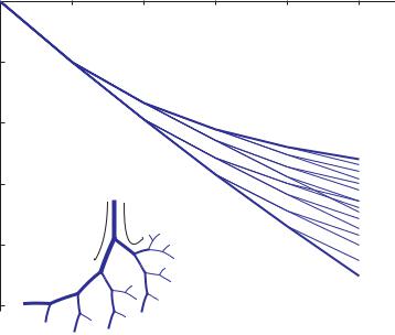
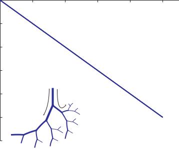
Fig. 9.2.5. Pressure distributions along paths from the root segment to all terminal segments of the 5-level tree structure shown in the inset. The two bold curves represent the pressure distributions along the two “bounding paths”, the pressure distributions along all other paths fall in between those two. The pressure falls linearly in each segment in accordance with the pressure drop in Poiseuille flow, but the magnitude of the drop depends on the radius of each vessel segment and on the amont of flow. Results in this figure are based on the assumption that the flow rate in a vessel segment is proportional to the square of its radius.

Similarly, the pressure distribution in the terminal branch segment with position coordinates 4, 16 is given by

streamwise distance X (normalized)

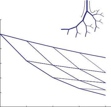
Fig. 9.2.6. Pressure distributions in the 5-level tree structure as in Fig. 9.2.5, but here the results are based on the assumption that the flow rate in a vessel segment is proportional to the fourth power of its radius. It is seen that under this assumption the pressure drops more steeply along the path of branches with the larger radii than it does along the path of branches with the smaller radii, which is somewhat unlikely on physiological or fluid dynamic grounds.

These two particular segments and the paths leading to them from the root segment of the tree are clearly singular in the sense that the path to segment

radius, and the linear relation between vessel length and radius, are not met exactly in the cardiovascular system but are met with considerable scatter as stated in the previous chapter and as data from the cardiovascular system indeed indicate [224, 215, 226, 106, 218, 220].

9.3 Pulsatile Flow in Rigid Branching Tubes

While pulsatile flow in a rigid tube is an idealized model of pulsatile flow in an elastic blood vessel as remarked at the end of the previous section, the results which the model produces provide important benchmarks for pulsatile flow in elastic tubes. Before we consider that problem, therefore, we continue to use the rigid tube model in this section to examine pulsatile flow in a tree structure consisting of rigid tube segments such as that considered for steady flow in Section 9.2.

From the previous chapter the key parameter that determines the properties of pulsatile flow in a rigid tube is the frequency parameter, also known as the Womersley number,

If the flow in a tree structure made up of many rigid tube segments is driven by an oscillatory input pressure of the form

then the frequency of oscillation ω in Eq. 9.3.1 for tube segments throughout the tree will be determined by the frequency of that input pressure. Assuming, also, that the fluid density ρ and viscosity μ in that equation remain constant throughout the tree, then the value of the frequency parameter Ω will change only with the radius a of tube segments within the tree.

To illustrate the variation of Ω along the 5-level tree structure considered in Section 9.2, taking the following property values

where a is the radius of the tube in centimeters. This expression can be used to map out the values of Ω along the 5-level tree structure in which the radii

308 9 Basic Unlumped Models

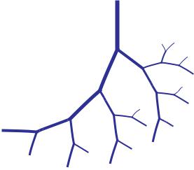
Fig. 9.3.1. Values of the frequency parameter Ω at di erent segments of the 5-level tree shown in the inset. The tree is based on a power law relation between flow rate and vessel radius, with power law index γ = 3.0 and bifurcation index α = 0.7. The values of Ω decrease most rapidly along the bounding path marked Ω2 consisting of branch segments with the smaller radii at each bifurcation, and most slowly along the other bounding path, marked Ω1. Values of Ω at other branch segments fall in between these two extremes.

of branch segments are determined by the power law relation between flow and radii used in Section 8.4.

Starting out with a = 0.2 cm as the radius of the root segment of the tree, which is representative of the radius of a main human coronary artery, the radii of subsequent branch segments are then given by Eqs.8.4.27,28 assuming the power law relation on which these equations are based. Values of the frequency parameter Ω obtained with these radii, and with the parameter values in Eqs.9.3.3-6 are shown in Fig. 9.3.1. In general the value of Ω decreases along any streamwise path from the root segment of the tree. It decreases most rapidly along the bounding path consisting of branch segments with the smaller radii at each bifurcation, and most slowly along the other bounding path. In a tree structure with a larger number of levels the values of Ω continue

Fig. 9.3.2. Values of the frequency parameter Ω in a tree with the same parameters as that in Fig. 9.3.1 but here the tree has 11 levels (marked 0 to 10). Values of Ω continue to decrease, ultimately reaching towards zero.

to decrease, reaching ultimately towards zero, as illustrated in Fig. 9.3.2 for an 11-level tree.

Based on values of the frequency parameter, the maximum flow rate reached within the oscillatory cycle in each tube segment within the tree, which we shall refer to simply as “peak flow”, can be calculated using Eq. 8.5.24 for the oscillatory flow rate qφ(t). In normalized form, this peak

The distribution of peak flow within the 5-level vascular tree is shown in Fig. 9.3.3. Because it is normalized in terms of the steady flow rate qs in Poiseuille flow (Eq. 9.3.8), this peak flow is a measure of how close the oscillatory flow at each point in time is to a Poiseuille flow driven by a pressure gradient equal to the value of the oscillatory pressure gradient at that point in time. Thus, a normalized peak flow of 1.0 represents an oscillatory flow in which the velocity profile at each point in time is a Poiseuille flow profile, while values less than 1.0 represent oscillatory flows in which peak flow does not quite reach the corresponding Poiseuille flow value. The results in