The Physics of Coronory Blood Flow - M. Zamir

320 9 Basic Unlumped Models

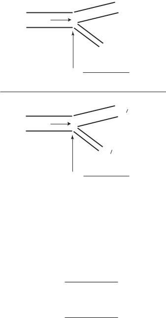
If wave reflections arise at a junction between two tubes denoted by A and B whose characteristic admittances are Y0A and Y0B , and if there are no further reflections at the downstream end of the second tube, as shown schematically in Fig. 9.5.1, then the reflection coe cient RA at the junction can be expressed in terms of the two characteristic admittances

But if there are wave reflections at the downstream end of the second tube then its admittance is now its e ective admittance YeA, and the expression for the reflection coe cient becomes

Similarly, at a bifurcation, since the combined admittance of the two branches is simply the sum of the two (hence it is convenient to use admittance

Fig. 9.5.1. The reflection coe cient RA at the junction between two tubes depends on the di erence between the characteristic admittances Y0A of the first tube and Y0B of the second if wave reflections are absent (top), or the di erence between the characteristic admittance Y0A of the first tube and the e ective admittance YeB of the second if wave reflections are present (bottom).

RB = 0

B

A

C

RC = 0

RA =

Y0A - (Y0B + Y0C)

Y0A + (Y0B + Y0C)

RB = 0

B

A

C

RC = 0

RA =

Y0A - (YeB + YeC)

Y0A + (YeB + YeC)

Fig. 9.5.2. The reflection coe cient RA at an arterial bifurcation depends on the di erence between the characteristic admittance Y0A of the parent vessel segment and the sum of the characteristic admittances Y0B , Y0C of the two branch segments if wave reflections are absent (top), or the di erence between the characteristic admittance Y0A of the parent vessel segment and the sum of the e ective admittance YeB , YeC of the two branch segments if wave reflections are present (bottom).

rather than impedance in the analysis of branching trees), then, as illustrated schematically in Fig. 9.5.2, in the absence of wave reflections at the downstream ends of the two branches we have

and in the presence of wave reflections

In a tree structure the e ective admittance of each vessel segment depends on wave reflections from all junction sites downstream of that segment. To calculate these, we may use Eq. 9.5.16 for the e ective admittance of the

324 9 Basic Unlumped Models

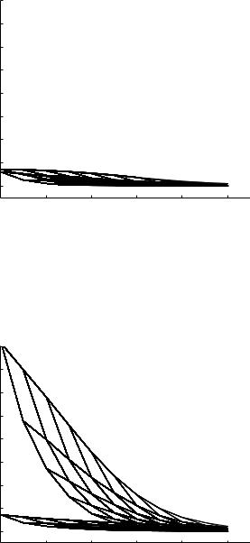
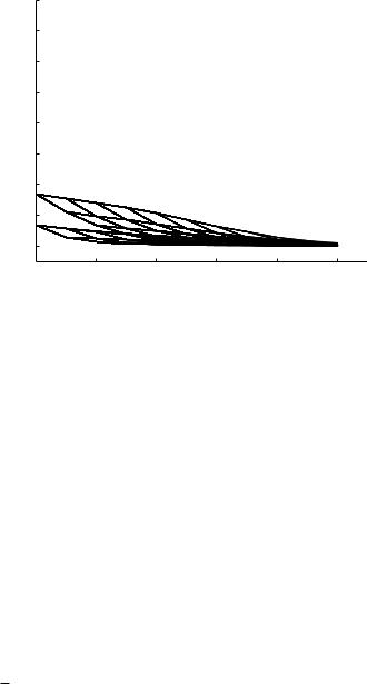
Fig. 9.5.5. Absolute values of the e ective (bold) and characteristic (thin) admittances at di erent levels of the 11-level tree model, as in Fig. 9.5.3 but here with a frequency of 10 Hz.

Fig. 9.5.6. Absolute values of the e ective (bold) and characteristic (thin) admittances at di erent levels of the 11-level tree model at a frequency of 1 Hz, as in Fig. 9.5.3, but here using a value of the wave speed c obtained from a solution of the pulsatile flow in an elastic tube for each vessel segment.

Fig. 9.5.7. Absolute values of the e ective (bold) and characteristic (thin) admittances at di erent levels of the 11-level tree model at a frequency of 5 Hz, as in Fig. 9.5.4, but here using a value of the wave speed c obtained from a solution of the pulsatile flow in an elastic tube for each vessel segment.

The di erence between the distribution of characteristic admittances and that of e ective admittances, which is due entirely to the e ects of wave reflections, is seen to be fairly large. Furthermore, because these e ects are cumulative, they reach their highest value at the root of the tree as observed in the figure.

The most important aspect of the results in Fig. 9.5.3 is that the e ects of wave reflections in this tree model are seen to produce higher admittance, and hence lower impedance, within the tree. This is particularly significant because the physical dimensions of the model are of the same order of magnitude as those in the coronary circulation, with wave-length-to-tube-length ratios well above 100 everywhere along the tree as illustrated in Fig. 9.4.3. This means that the direct e ects of wave propagation, due to the di erence between pulsatile flow in an elastic tube and that in a rigid tube, are negligibly small as shown in Figs. 8.6.4, 5, but the indirect e ects, due to wave reflections, are very large and far from being negligible.

Indeed, while the direct e ects of wave propagation diminish at higher values of λ as observed in Figs. 8.6.4, 5, the reverse is true for the indirect e ects, namely the e ects of wave reflections. This is because the relation between the wave length λ and the frequency f (in cycles per second) is

326 9 Basic Unlumped Models

where c is the wave speed. Thus, all else being unchanged, higher frequencies are associated with lower wave lengths and hence lower values of wave-length- to-tube-length ratios λ. In Section 8.6 we saw that this produces more significant direct e ects of wave propagation, in terms of direct changes in the flow field, than those in a rigid tube. By contrast, the indirect e ects of wave propagation due to wave reflections, are less significant at higher frequencies as shown in Figs. 9.5.4, 5 where the calculations for the 11-level tree model are repeated at frequencies of 5 and 10 Hz. Compared with the results at 1 Hz in Fig. 9.5.3, it is seen that the di erence between e ective and characteristic admittances is much higher at 1 Hz. This is particularly significant in the physiological system because the fundamental frequency of the composite pressure wave (in humans), which represents the frequency of the largest harmonic component of the composite wave, is very close to 1 Hz. The higher frequencies are associated with the much smaller harmonics of the composite wave.

The situation is somewhat more complicated, however, because the wave speed c in Eq. 9.5.23 is also a function of frequency. In Figs.9.5.3-5 this was simplified by taking c = c0 where c0 is the constant Moen-Korteweg wave speed. In order to account for this e ect, the calculations of characteristic admittances in these figures must be repeated by using a value of c obtained from the solution for pulsatile flow in an elastic tube for each vessel segment.

Fig. 9.5.8. Absolute values of the e ective (bold) and characteristic (thin) admittances at di erent levels of the 11-level tree model at a frequency of 10 Hz, as in Fig. 9.5.5, but here using a value of the wave speed c obtained from a solution of the pulsatile flow in an elastic tube for each vessel segment.

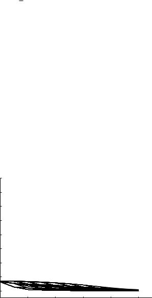
Fig. 9.5.9. Absolute values of the e ective (bold) and characteristic (thin) admittances (which in this case coincide) at di erent levels of the 11-level tree model at a frequency of 1 Hz and c = c0, as in Fig. 9.5.3, but here using a square law (γ = 2) for the hierarchy of radii at di erent levels of the tree. The law produces what is generally referred to as “impedance matching” at arterial bifurcations because it implies that the impedance of the parent vessel is equal to the combined impedance of the two branches. Under these conditions the e ective admittances are everywhere the same as the corresponding characteristic admittances, which means that the e ects of wave reflections are entirely eliminated. It is important to note that impedance matching requires not only γ = 2 but also c = c0.

The results are shown in Figs.9.5.6-8. This “refinement” produces essentially the same results, though with even higher e ects of wave reflections.

Finally, the results in Figs.9.5.3-8 are all based on a tree model in which the hierarchy of vessel radii follows the cube law discussed in Section 8.4, namely γ = 3.0. An interesting case to consider is a model in which γ = 2.0 and c = c0. The results are shown in Fig. 9.5.9, where the e ects of wave reflections are seen to be totally absent and the distributions of characterisic and of e ective admittances are identical. The result shown is for a frequency f = 1 Hz, but the same results are obtained for other frequencies.

The reason for these rather singular results is that when the power law index γ = 2.0, the sum of cross-sectional areas of the two branches at a bifurcation is equal to the cross-sectional area of the parent vessel, that is (Eq. 8.4.25)

328 9 Basic Unlumped Models

Fig. 9.5.10. Absolute values of the e ective (bold) and characteristic (thin) admittances at di erent levels of the 11-level tree model, as in Fig. 9.5.9, but here using a value of the wave speed c obtained from a solution of the pulsatile flow in an elastic tube for each vessel segment, instead of c = c0 on which the results in Fig. 9.5.9 are based. The results show that impedance matching does not occur in this case because it requires γ = 2 and c = c0.

Now, using Eq. 9.5.5, the characteristic admittances of the three vessels are given by

πa2

Y0A = A (9.5.26)

ρcA

πa2

Y0B = B (9.5.27)

ρcB

πa2

Y0C = C (9.5.28)

ρcC

and the corresponding characteristic impedances are given by

If c = c0, which is assumed to be the case in Fig. 9.5.9, it is clear that in view of Eq. 9.5.25 the three admittances and three impedances are related by

which constitute what is generally referred to as “impedance matching” at the bifurcation, meaning that the propagating wave does not encounter any change of impedance (or admittance) as it crosses the bifurcation and hence there are no wave reflections at the junction. Since this is true at all bifurcations of the 11-level tree model, with γ = 2, it follows that no wave reflections arise throughout the tree and hence the e ective admittances are everywhere the same as the corresponding characteristic admittances as observed in Fig. 9.5.9.

It has been suggested that “square law” conditions (γ = 2.0) prevail in the first branching levels of the aorta [230, 201], and that this is a deliberate design feature of the cardiovascular system which has the advantage of avoiding wave reflection e ects at these levels of the vascular tree. This may indeed be the case in the larger vessels of the cardiovascular system where values of the frequency parameter Ω are su ciently high that the wave speed is close to the constant Moen-Korteweg wave speed (Fig. 8.6.2) which the conditions for impedance matching require. However, in the coronary circulation where the values of Ω are typically much lower (Fig. 9.3.2) these conditions are not met, and as we saw in Section 9.4, the wave speed in fact is significantly di erent from c0 (Fig. 9.4.1). Thus, strictly, for application to the coronary circulation the calculations on which the results of impedance matching in Fig. 9.5.9 are based must be repeated using the actual value of c obtained from a solution for pulsatile flow in an elastic tube for each vessel segment. The results are shown in Fig. 9.5.10 where it is seen clearly that impedance matching does not occur at the junctions, and e ective admittances are significantly di erent from the corresponding characteristic admittances in most of the tree structure.

9.6 Pulsatile Flow in Elastic Branching Tubes

A principal tool in the analysis of pulsatile flow in branching elastic tubes is the “pressure distribution” along a tube segment within the branching tree structure, which we defined earlier as the amplitude of time oscillations in pressure at di erent points along that segment. In the absence of wave reflections the pressure distribution is uniform at a normalized value of 1.0 along the entire length of the tube segment (Fig. 8.7.2), but in the presence of wave reflections this is no longer the case, as illustrated in Figs.8.7.5-9. Thus, in