The Physics of Coronory Blood Flow - M. Zamir

360 9 Basic Unlumped Models

segments, the total opposition to pulsatile flow registered at entry into the tree is referred to as “input impedance”. One part of this opposition depends on the elasticity and other geometric properties of the tube segments as well as on the frequency of the oscillatory flow and is referred to as “characteristic” impedance. Another part is due to wave reflections and it depends on the succession of local impedances at vascular junctions as well as on the frequency of the oscillatory flow. When this part is included in the total opposition to pulsatile flow it is referred to as “e ective” impedance. Similar terminology is used for admittance. Only under very special circumstances is the e ective impedance in a vascular tree the same as the characteristic impedance. These circumstances require that the characteristic impedance of the parent vessel at every vascular junction be the same as the combined characteristic impedance of the two daughter segments, which is generally referred to as “impedance matching”, and that the wave speed be constant throughout the tree and equal to the Moen-Korteweg wave speed. These circumstances do not occur in the coronary circulation.

In a tree model consisting of elastic tube segments and having dimensions comparable with those of the human coronary arterial tree, pulsatile flow is associated with significant wave reflection e ects that produce a negative pressure gradient along the tree that actually aids rather than impedes the flow. If the dimensions of the tree are made comparable with those of the systemic arterial tree, this trend is reversed initially to produce a positive pressure gradient, consistent with the well known “peaking” phenomenon in the descending aorta, and then becomes negative again towards the periphery.

A cardiac pressure wave representing input pressure into a tree model consisting of elastic tube segments and having dimensions comparable with those of the human coronary arterial tree, is generally “blunted” or “flattened” as it progresses from the root segment of the tree to the periphery. This is the reverse of the “peaking” phenomenon observed in the descending aorta, the di erence being due to the di erent scales of the coronary and systemic circulations, but the change in the form of the wave in both cases is due to wave reflections. In the systemic circulation the wave would be blunted by viscous dissipation as it travels along the descending aorta, but instead it peaks because of wave reflections coming from downstream. In the coronary circulation model being considered here the wave is blunted with or without the e ects of viscosity (by using c or c0) thus the blunting is due largely to wave reflections.

10

Dynamic Pathologies

10.1 Introduction

The dynamics of the coronary circulation are under strict regulation, mediated by several neural and humoral control mechanisms [83, 128]. While a great deal has been learned about the isolated e ects of certain humoral agents or neural stimuli, a full understanding of the feedback loops associated with these mechanisms does not exist at present. These aspects of the coronary circulation have yet to be integrated into a unified model of the dynamics of the system.

In the absence of an integrated model, it is not unreasonable to assume that the regulatory mechanisms of the system will aim to keep it in a mode of operation in which its dynamics are “optimal” in some way. And if the parameter values associated with these optimal dynamics are changed, whether by disease or clinical intervention, the dynamics of the system will then be less than optimal. They will be “pathological” in the sense of being away from the normal dynamics of the system, and it is in this sense that we use the term “dynamic pathology” in this chapter.

A dynamic pathology is not unlike a structural or a functional pathology in a tissue or organ, but it deals specifically with dynamics. Furthermore, it deals with the dynamics of an integrated system as a whole, such as the dynamics of the coronary circulation as a whole. Thus, an atherosclerotic lesion in a coronary artery is a vascular pathology but the ultimate significance of this lesion lies in the dynamic pathology which it produces. The ultimate significance of the lesion lies in the way it a ects the dynamics of the coronary circulation as a whole, and in particular in the way it a ects the ultimate goal of the coronary circulation to provide the heart with su cient blood supply. If the occlusive progression of a lesion is su ciently slow, so that the occlusion is compensated for by vascular restructuring, then the dynamic pathology may be minimal or nonexistent. Thus, the presence of vascular pathology does not necessarily imply the presence of dynamic pathology. The tenet of this book is that the reverse of this statement is also true, namely that the absence of

362 10 Dynamic Pathologies

vascular pathology in the coronary circulation does not necessarily imply the absence of dynamic pathology.

Arrhythmia, in all its forms, is a familiar example of a dynamic pathology. It a ects the harmony between the pumping rhythm of the heart and the compliance of the aorta, thereby a ecting cardiac output and hence the dynamics of the systemic circulation. Similarly, a disruption in the harmony between the pulsatile rhythm of the input pressure driving the flow into the coronary circulation, the pulsatile rhythm of the contracting cardiac muscle and its e ect on coronary vessels imbedded within it, and the combination of wave propagation and wave reflections within the coronary vascular tree, will lead to dynamic pathology in the coronary circulation. Anyone who has pushed a child on a swing in the park will know the exquisite harmony required between the timing of the push and the rhythmic momentum of the swing. Any disruption in that harmony will cause the swing to lose rather than gain momentum, thus producing a dynamic pathology. The analogy is quite pertinent and we shall use it again later. Any disruption in the harmony between the several factors involved in the dynamics of the coronary circulation will reduce the e ciency of coronary blood flow and thereby produce dynamic pathology.

While an integrated model of the coronary circulation that can deal with these dynamic issues and with dynamic pathologies in the system does not exist at present, the lumped and the unlumped models introduced in previous chapters, though incomplete, can provide tools for a useful prelude to dealing with these issues. The models can be used to assess the consequences of a change in diameters or mechanical properties of the vessels involved or in the frequency of oscillation, to then speculate on the possible role such changes might play in an integrated model of the coronary circulation. Alternatively, results of lumped and unlumped models, though incomplete, can be used in combination with known dynamic features of the coronary circulation to speculate on possible dynamic factors in coronary heart disease. We follow some of these lines in this concluding chapter of the book, which is therefore largely speculative in scope.

10.2 Magic Norms?

While the goal of uncovering the full range of dynamics of the coronary circulation may be out of reach, a more modest goal is that of finding “ideal” or “normal” modes of operation of the system, modes of operation in which the dynamics of the system appear to be particularly simplified or optimal in some sense. We shall refer to these loosely as “magic norms” of the system in the sense that they may represent modes of operation for which the system is designed (or towards which the system has evolved).

10.2 Magic Norms? 363

Fig. 10.2.1. Oscillatory pressure (solid) and flow (dashed) in an RLC system in series. The flow rate is “R-scaled” such that the pressure and flow curves become identical under pure resistance, that is when L and C are absent. In the presence of L and C, however, the system has a magic norm in which it behaves as if L and C are absent. If the value of the inertial time constant tL is taken as 0.1 s, the magic norm conditions occur when the value of the capacitive time constant tC is 0.0253 s. Any deviation from this value moves the system away from this mode, as indicated by the departure of the flow curve away from the pressure curve.

Thus, a lumped or unlumped model of the coronary circulation may not embody the full range of dynamics of the system, but it may embody some of its magic norms. While the model may be incomplete in terms of the range of parameters on which it is based, it may point to modes of operation of the system in which a unique combination of the values of these parameters produce remarkably simplified dynamics.

An example from another area of application may illustrate the point. The dynamics of a pendulum depend on several parameters such as length, weight, and any driving forces. The di erential equations governing these dynamics, as well as their solutions, are fully known in even the most complicated cases. When a child sits on a swing in the park for the first time, however, the child does not know that the swing is in fact a pendulum with fully known dynamics, yet he or she very quickly discovers the magic norm of the system. The child soon discovers how to use his or her body weight to drive the swing to higher and higher altitudes. He or she soon learns that the amount and exquisite timing of the applied body force is crucial to attaining the magic norm, and reaching the ideal conditions under which the system operates.

364 10 Dynamic Pathologies

Fig. 10.2.2. Oscillatory pressure (solid) and flow (dashed) in Lumped Model 2 of Section 7.4 whose composition in the notation of that section is {{R1+L}, {R2+C}}. A magic norm occurs when λ = R2/R1 = 1.0 and tL = tC = 0.2 s whereby the system behaves as if L and C were absent, and the pressure and R-scaled flow curves again become identical. Other values of λ (shown) move the system away from the magic norm.

Any deviation from the precise timing or the precise force moves the system away from its magic norm.

While the dynamics of the coronary circulation may be several orders of magnitude more complicated than the dynamics of a swing, the example is pertinent in the sense that we are somewhat in the position of the child who does not know the equations governing the full dynamics of the system, yet we may recognize conditions under which the dynamics of the system appear to be ideal in some sense.

The first example of a magic norm was actually found in Section 4.8, where under certain circumstances the inertial and the capacitive e ects of the RLC system were found to “cancel” each other and produce zero reactance. These conditions were found to occur when the value of the capacitive time constant tC (= CR) and the value of the inertial time constant tL (= L/R) were such that (Eq. 4.8.22)

10.2 Magic Norms? 365

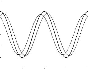
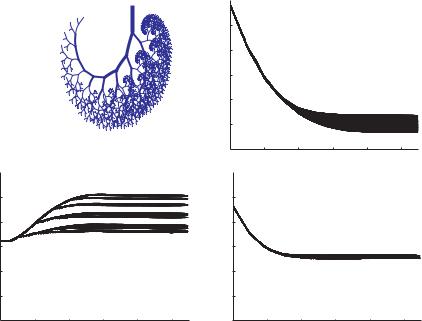
Fig. 10.2.3. Propagation of the cardiac pressure wave along the 11-level tree model. The input wave, shown in bold, would normally be modified as it progresses along the tree structure, but a “magic norm” occurs when the wave speed c is equal to the Moen-Korteweg wave speed c0 and the value of the power law index γ is 2.0 whereby the wave remains unchanged. Departure from any of these values moves the system away from this magic norm. The thin curves indicate the changed form of the wave as it travels in that case.

where ω is the frequency of oscillation of the driving pressure, R is resistance, L is inductance, and C is capacitance. Under this unique combination of values the RLC system behaves as if L and C do not exist, thus the relation between pressure and flow is particulary simple and is the same as that in the presence of resistance R only, namely

where q(t) is the oscillatory flow rate and Δp(t) is the oscillatory driving pressure. Thus, if the flow rate is multiplied by R, the resulting “R-scaled” flow rate becomes identical with the driving pressure, as illustrated in Fig. 10.2.1.

For the purpose of illustration, in Fig. 10.2.1 the value of tL is taken as 1 s and the frequency of oscillation is taken as 1 Hz, thus ω = 2π rad/s. This means that the magic norm conditions occur when tC = 1/ω2 = 0.0253 s

366 10 Dynamic Pathologies

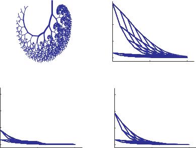
Fig. 10.2.4. E ects of “vasoconstriction” and “vasodilatation”, as defined in the text, on the values of admittance within the 11-level tree model, compared with the “normal” case, at a frequency of 1 Hz. The two conditions produce significant changes in the distribution of admittance and hence in the dynamics of pressure and flow within the tree model.

as required by Eq. 10.2.1. The “magic” in this magic norm is illustrated in Fig. 10.2.1 where it is seen that any small departure from this particular value of tC leads to a departure from the ideal relation between pressure and flow.

As discussed in Section 4.7, an appropriate value of tL for the coronary circulation is not known, if indeed a single such value is appropriate at all. Nevertheless, the results in Fig. 10.2.1 are valuable in providing a hint at the relative values of the two time constants, as provided by Eq. 10.2.1. Because of the great simplicity of the pressure-flow relations under these conditions, it is highly tempting to speculate that the coronary circulation may be designed to operate with values of the two time constants that are close to those provided by Eq. 10.2.1. It would then follow that any departure from these ideal values would be functionally undesirable in the sense that it would disrupt the ideal relation between pressure and flow. As in the case of the child on a swing, any departure from the perfect timing of the force which the child applies with his or her body leads to disruption in the ideal operation of the swing.

While the magic norm in Fig. 10.2.1 is based on a driving pressure consisting of a single harmonic through a simple RLC system in series, similar

368 10 Dynamic Pathologies

Fig. 10.2.6. E ects of “vasoconstriction” and “vasodilatation”, as defined in the text, on the pressure distribution within the 11-level tree model, compared with the “normal” case as in Fig. 10.2.5 but here at a frequency of 10 Hz. The e ects of the two conditions on the pressure distribution are clearly more dramatic at the higher frequency.

magic norm occurs when the value of the power law index γ is 2.0 and the wave speed c is taken equal to the Moen-Korteweg wave speed c0. Any departure from these conditions leads to departure from the magic norm, as illustrated in Fig. 10.2.3.

It must be remembered, of course, that the coronary circulation is not a simple RLC system nor an idealized tree model, thus the parameter values for the magic norms described here cannot be applied directly to the coronary circulation. The ultimate value of these results lies in pointing out that the coronary circulation very likely has its own magic norm or norms and that any disruption in the conditions required for these norms will move the system away from its optimal dynamics. Such disruptions may occur as a result of vascular disease or aging, which would change the mechanical properties of the vessel wall or constrict the lumen available for the flow, or as a result of clinical intervention, whether by drugs or surgery. To illustrate this more succinctly, we finish this section by considering the 11-level tree model with architecture on the scale of the coronary circulation as was done in Chapter

10.2 Magic Norms? 369

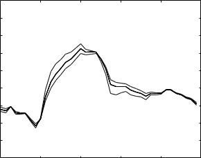
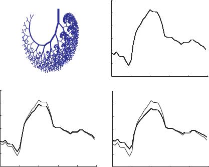
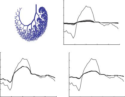
Fig. 10.2.7. Propagation of the cardiac pressure wave along the 11-level tree model, the input waveform being shown in bold, while the thin curves indicate the changed form of the wave as it travels in that case. The three panels show the e ects of “vasoconstriction” and “vasodilatation”, as defined in the text, compared with the “normal” case at a frequency of 1 Hz.

9. Then we consider two scenarios in which the peripheral 6 levels of the tree are either constricted, with vessel diameters reduced by 50%, or dilated, with vessel diameters increased by 50%, while the elasticity of the same vessels is reduced to the e ect that the vessels become more rigid, with Young’s Modulus increased from 107 to 109 dyn/cm2. While the two scenarios are highly idealized, we shall refer to them loosely as conditions of “vasoconstriction” and “vasodilatation”, respectively, suggesting not that they replicate the corresponding physiological conditions but that they may be relevant to them. E ects of these scenarios on admittance or pressure distribution or on the form of the propagating wave within the tree structure are shown in Figs.10.2.4-9.