The Physics of Coronory Blood Flow - M. Zamir

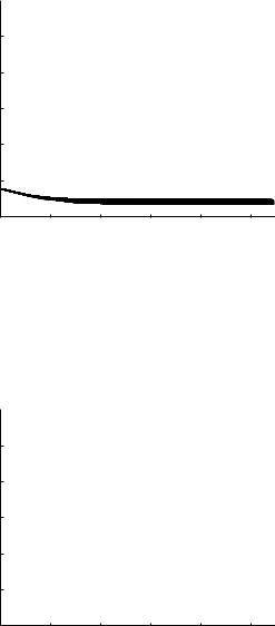
344 9 Basic Unlumped Models

pressure”, may be considered reasonably accurately as the oscillatory input pressure for the coronary circulation. In other words, the cardiac pressure wave may be taken as the “input pressure” pin(t) at the root segments of the two main coronary arterial trees, with the role and significance of pin(t) as described in Section 8.7 and used in the previous two sections. However, in those sections pin(t) was taken as a single harmonic function, meaning that it has the form of a simple sine or cosine function. In the present section we consider pin(t) to be a composite wave that has the form of the cardiac pressure wave shown in Fig. 9.7.1.

Fig. 9.7.1. The composite pressure wave considered as the input pressure driving coronary blood flow. Of ultimate interest is to determine the way in which the form of the wave is modified as it travels down the coronary vasculature. To do so requires that the wave be decomposed into its harmonic components and then recomposed in terms of its modified components.

As discussed in Section 8.7, when the oscillatory input pressure pin(t) at entry to an elastic tube is a single harmonic, the pressure wave which it produces within the tube is also a single harmonic function of time but with amplitude which depends on position x within the tube. The way in which the amplitude varies with x is what we have called the “pressure distribution” along the tube. When the oscillatory input pressure pin(t) is a composite wave, these concepts cannot be applied to the composite wave as a whole because the notion of an amplitude does not apply to a composite wave. But the concepts of amplitude and pressure distribution do apply to the individual harmonics of the composite wave.

Thus, if the cardiac wave in Fig. 9.7.1 is decomposed into its individual harmonics as discussed in Chapter 5, the pressure distribution associated with each harmonic can be obtained as in the previous section. This pressure distribution represents the amplitude of the propagating wave associated with that particular harmonic at di errent positions x along each tube segment and along the tree as a whole. At a particular position x, therefore, the collective amplitudes associated with all the harmonics of the composite cardiac wave represent the amplitudes of the individual harmonics of the modified form of the composite wave at that position. The modified form of the wave is thus determined from the collective amplitudes at that position by simply recomposing the harmonics associated with these amplitudes, using the Fourier analysis techniques discussed in Chapter 5.

In fact, since the pressure distributions obtained in the previous section were all normalized so that the input pressure at entry has an amplitude of 1.0, then the same analysis and results can be applied to all the harmonics of the composite cardiac pressure wave if each harmonic is first normalized so that the input pressure at entry associated with it has a normalized value of 1.0, and then “denormalized” when the modified harmonics are put together to recompose the modified composite wave.

The end results of this exercise provide a picture of the evolution of the composite pressure wave as it travels along di erent paths within the tree structure. These results are strongly linked to results obtained in the previous section because the evolution of the composite wave along a given path indeed consists of the aggregate pressure distributions associated with its individual harmonics along that path. In a graphical presentation of the results, however, only one path can be considered at a time because the full form of the wave must be presented at di erent points along the path. For this reason we shall focus on the evolution of the wave along the two bounding paths defined in Fig. 9.6.1. Since the pressure distributions along these two paths represent the bounds on the pressure distribution within the tree as a whole, the evolution of the composite pressure wave along these two paths will represent similar bounds on the evolution of the composite pressure wave along the tree as a whole.

Computed evolutions of the composite pressure wave along the two bounding paths of the 5-level tree model at three di erent frequencies are shown in Figs.9.7.2-7. At each frequency, the evolution of the composite wave along a given path can be interpreted in terms of the corresponding pressure distribution along that path obtained in the previous section. Thus, the pressure distribution along path-1 of the 5-level tree model in Fig. 9.6.2 of the previous section indicates that at a frequency of 10 Hz the amplitude of a harmonic wave starting with a normalized amplitude of 1.0 is modified by wave reflections so that its values at di erent points along the path are as indicated by that curve. Since the values of the modified amplitude are everywhere below the initial value of 1.0 and continue to decrease along the path, it follows that the same will be true of the individual harmonics of a composite wave

346 9 Basic Unlumped Models

travelling down the same path. Thus, because the amplitudes of its harmonic components are diminishing as it travels, the composite wave will be “flattened”, or “blunted”, as it progresses along the path, as is indeed observed in Figs. 9.7.2, 3 where the frequency is 10 Hz as it is in Fig. 9.6.2.

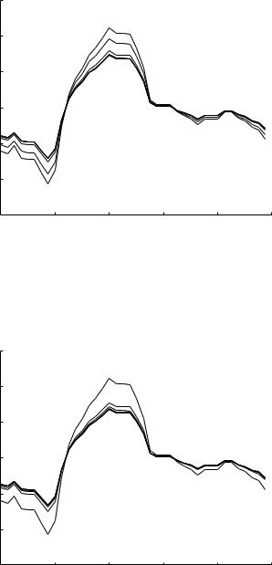
Fig. 9.7.2. Evolution of the composite cardiac pressure wave as it travels down path- 1 of the 5-level tree model. The top bold curve represents the input pressure wave at entry while the thin curve next to it in sequence represents the form of the pressure wave that actually prevails at entry, which illustrates graphically that the two are di erent because of wave reflections returning from downstream as discussed in Section 9.6 (Eqs.9.6.13,14). Thin curves further down in sequence represent modified forms of the wave at higher levels of the tree. There is thus a general “flattening”, or “blunting”, of the wave as it progresses, consistent with the corresponding pressure distribution along the same path shown in Fig. 9.6.2.

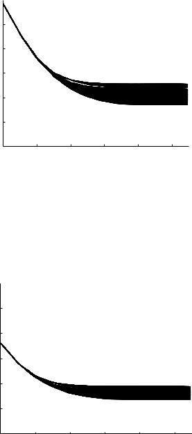
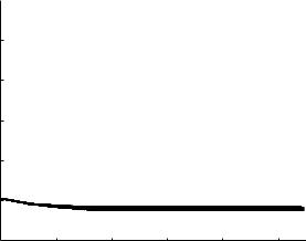
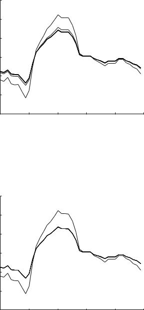
At the lower frequencies of 5 Hz and 1 Hz, the evolutions of the composite pressure wave are shown in Figs. 9.7.4–7 and they can be interpreted in the same way in relation to the corresponding pressure distributions in Figs.9.6.3,4. In particular, at the lowest frequency of 1 Hz, the pressure distribution in Fig. 9.6.4 shows not a gradual but a uniform drop in the amplitude of harmonic components, therefore leading to the abrupt change in the form of the composite wave observed in Figs. 9.7.6, 7.

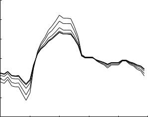
Evolutions of the composite cardiac pressure wave along the 11-level tree model are shown in Figs.9.7.8-13, to be interpreted in terms of the corresponding pressure distributions in Figs.9.6.5-7. In particular, results in Figs. 9.7.8, 9 indicate that at the highest frequency of 10 Hz some “peaking” of the wave-

Fig. 9.7.7. Evolution of the composite cardiac pressure wave as it travels along the 5-level tree model as in Figs. 9.7.2, 3 but here at a frequency of 1 Hz, consistent with the corresponding pressure distribution along the same path shown in Fig. 9.6.4.

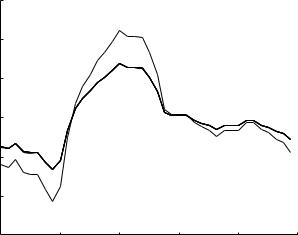
form occurs initially. This is consistent with the pressure distributions in Fig. 9.6.5 where it is seen that at the root segment of the tree the normalized pressure amplitude is higher than the benchmark of 1.0. Peaking of the pressure waveform due to wave reflections is known to occur in the systemic circulation as the cardiac pressure wave travels down the abdominal aorta. Results obtained in this section so far indicate that in the coronary circulation, because of the much higher wave-length-to-tube-length ratios, wave reflections lead mostly to a flattening of the pressure waveform, which is the reverse of peaking. But the results in Figs.9.7.8,9 demonstrate that peaking may occur in the coronary circulation too, though only locally and under limited circumstances. Indeed, the phenomenon is no longer present at higher levels of the tree at 10 Hz, and not present at all at the lower frequencies of 5 Hz and 1 Hz as seen in Figs.9.7.10-13.

To pursue the peaking phenomenon a little further, and to compare the evolution of the pressure waveform on the scale of the coronary circulation with that on the scale of the systemic circulation, the dimensions of the 11level tree model are increased accordingly as before, with the root segment of the tree being given a diameter of 25 mm. Results are shown in Figs.9.7.14-16. Compared with the corresponding results on the scale of the coronary circulation (Figs. 9.7.8, 10, 12), the peaking phenomenon is clearly more prominent here than it is on the scale of the coronary circulation. Also, here the evolu-