The Physics of Coronory Blood Flow - M. Zamir

138 4 Forced Dynamics of the RLC System

Broadly speaking, impedance is the total impediment to oscillatory flow in the presence of inductance and capacitance e ects. We do not use the term “resistance” here, because that term is generally reserved for the e ects of viscosity in steady as well as in oscillatory flow. Essentially, impedance embodies both the resistance R and the reactance S discussed in the previous section.

There is a fundamental di erence between impedance and the familiar viscous resistance which makes it important not to confuse the two. Viscous resistance dissipates energy which must be replaced constantly from a source of driving energy (pump). Reactance, on the other hand, as seen in the previous section, presents an impediment to flow in the sense of a ecting the amplitude and phase of the flow wave, but it does not actually dissipate the flow energy. Under reactive e ects flow energy is only exchanged between pressure and kinetic energy, as when fluid is accelerated or decelerated, or between pressure inside the capacitive balloon and elastic energy in its walls. Impedance embodies these exchanges as well as the dissipative viscous resistance and therefore it would be inappropriate to describe it simply as “resistance to flow”.

The primary reason for using the concept of impedance is that it provides a link beween flow and pressure drop in oscillatory flow, in the same way that resistance provides that link in steady flow. Thus, for steady flow in a tube we have the basic result from Section 2.4 that the flow rate q is simply equal to the pressure drop Δp divided by the resistance R, that is (Eq. 2.4.3)

In oscillatory flow the concept of impedance is introduced in order to be able to write the relation between flow and pressure drop in a similar way, namely

where IM P is used here as a generic label for impedance until it can be defined more accurately.

In the solution obtained in the previous section the driving oscillatory pressure drop was of the form (Eq. 4.8.2)

while the the flow rate was found to be of the form (Eq. 4.8.5)

where Δp0 is a constant representing the amplitude of the driving oscillatory pressure drop, ω is the (angular) frequency of oscillation, R is resistance, S is reactance, and θ is the phase angle between the pressure and flow waves, as defined in the previous section.

From Eqs.4.9.3,4 it is not possible to write the relation between q(t) and Δp in the form of Eq. 4.9.2. This is because impedance a ects both the amplitude

and the phase angle of the flow wave, and these e ects appear separately in

√

Eq. 4.9.4. The amplitude e ect is represented by the term R2 + S2, while the phase angle e ect is represented by the angle θ. This suggests that impedance itself has an amplitude and phase, which in turn suggests that impedance is a complex quantity with a real and an imaginary part. This indeed turns out to be the case as we shall see below.

To reach this result we begin with a driving pressure drop in complex form, as was done in previous sections, namely

A steady state solution with this form of the pressure drop was obtained in details in Section 4.4 (Eqs.4.4.6,9), namely

Using these, the equation for the flow rate (Eq. 4.9.6) can then be put in the form

Eq. 4.9.10 is a relation between flow rate and pressure drop in the basic form of Eq. 4.9.2, therefore we identify Z as the impedance (IM P ) in that equation. Furthermore, as anticipated earlier, Z is a complex quantity as defined in Eq. 4.9.11, with the resistance R as its real part and the reactance S as its imaginary part. It is known as “complex impedance”.

We note from Eq. 4.9.11 that the amplitude and phase of Z are respectively

140 4 Forced Dynamics of the RLC System

which we recognize as the e ects of impedance on the amplitude and phase of the flow wave, as discussed earlier in this section.

To see this more clearly we now reproduce the result in Eq. 4.9.4 which represents the flow rate when the driving pressure drop is a cosine function (Eq. 4.9.9), which is equivalent to the real part of the complex pressure drop in Eq. 4.9.5, that is

The flow rate corresponding to this pressure drop is therefore the real part of the complex flow rate in Eq. 4.9.9, that is

The last expression is identical with the result in Eq. 4.9.4.

Thus, complex impedance o ers an elegant way of representing the e ects of impedance on both the amplitude and phase of the pressure wave. It also makes it possible to maintain the simple relation between pressure drop and flow, namely that in Eq. 4.9.10.

Indeed, because of the simple relation between q and Δp in Eq. 4.9.10, the analysis of several impedances in series or in parallel remains as simple as the analysis of several resistances in series or in parallel.

For impedances Z1, Z2, Z3 in series, using Eq. 4.9.10 with q as the common

Then, since the total pressure drop is the sum of the partial pressure drops, we find

142 4 Forced Dynamics of the RLC System

Note that the partial impedance of reactance, namely Z4, is defined as the sum of the partial impedances of inductance and capacitance when these elements are in series, therefore Z4 cannot be used when the two elements are in parallel. Instead, we may define

which is identical with the result in Eq. 4.9.44.

These are standard results in electric circuit theory, and they have been used extensively in the analysis of lumped models of the coronary circulation. We shall return to them in Chapter 6.

4.10 Summary

The dynamics of the coronary circulation are “forced” in the sense that they are driven by an external force. In free dynamics, the system’s behaviour depends on the internal characteristics only. In forced dynamics, by contrast, the behaviour of the system depends on these characteristics as well as on the form of the external driving force.

Free dynamics of the RLC system are governed by the homogeneous part of the solution of the governing equation, which depend on the characteristic properties of the system only. Forced dynamics are governed by the full solution of the equation, including the homogeneous part as well as the particular part of the solution, the so-called “particular solution”, which depends on the form of the external driving force.

When the pressure drop Δp driving the forced dynamics of the RLC system is expressed in the form of a complex exponential function, the solution of the governing equation produces two solutions at once: one corresponding to Δp being a sine function and the other to Δp being a cosine function.

In overdamped forced dynamics of the RLC system in series, under an oscillatory driving pressure, the flow begins with a “transient state” in which it

moves from a prescribed initial value to a “steady state” in which it oscillates in tandem with the driving oscillatory pressure. Overdamping occurs when (4tL/tC ) < 1.0 which, all else being the same, corresponds to a su ciently high value of the capacitance C, which in turn corresponds to a more elastic balloon that absorbs the filling without recoil.

In underdamped forced dynamics of the RLC system in series, under an oscillatory driving pressure, flow begins with a “transient state” in which it moves rather erratically to a “steady state” in which it oscillates in tandem with the driving oscillatory pressure. Underdamping occurs when (4tL/tC ) > 1.0 which, all else being the same, corresponds to a su ciently low value of the capacitance C, which in turn corresponds to a less elastic balloon that recoils in the initial phase.

In critically damped forced dynamics of the RLC system in series, under an oscillatory driving pressure, the flow begins with a “transient state” in which it moves most expediently to a “steady state” in which it oscillates in tandem with the driving oscillatory pressure. Critical damping is a singular scenario which occurs when (4tL/tC ) = 1.0. All else being equal, it corresponds to a unique value of the capacitance C that lies precisely between the overdamped and underdamped values.

Lumped model analysis of the coronary circulation is based on only the steady state dynamics of the system, transient state dynamics are neglected. The time required for the system to complete the transient state is di cult to estimate, yet it is clearly of clinical importance because it represents the time it would take the system to recover from a dynamic disturbance.

There are singular circumstances under which the reactance of the RLC system vanishes and the system behaves as if the inductance and capacitance do not exist. These circumstances are created by specific combinations of values of the inertial and capacitive time constants. Since the dynamics of the RLC system in series do not accurately represent the dynamics of the coronary circulation, these specific values of the time constants may not be directly relevant to the dynamics of the coronary circulation. However, the mere existence of these unique circumstances in the dynamics of the RLC system suggests strongly that similar circumstances may exist in the dynamics of the coronary circulation and that the system may normally operate at or near these ideal conditions.

Impedance is the total impediment to pulsatile flow, embodying the effects of capacitance and inductance as well as the familiar e ect of viscous resistance. Analytically, impedance is a complex quantity of which the real part represents the viscous resistance while the imaginary part represents the reactance which in turn represents the combined e ects of capacitance and inductance. In its complex form, impedance conveniently represents that ratio of pressure over flow in pulsatile flow in the same way that resistance represents that ratio in Poiseuille flow.

5

The Analysis of Composite Waveforms

5.1 Introduction

The oscillatory pressure drops used in all previous chapters have been of a particularly simple form, namely that of a trigonometric sine or cosine function. These waveforms have specific properties that make them particularly useful for the study of general dynamics of RLC systems such as those examined in previous chapters. However, the ultimate aim of these studies, in the context of the coronary circulation, is to examine the dynamics of RLC systems under oscillatory pressure drops of more general forms, in particular the forms of pressure waves generated by the heart. In what follows we shall refer to these generically as “composite” wave forms.

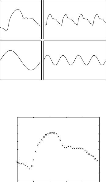
An example of a composite waveform is shown in Fig. 5.1.1, compared with a simple sine wave. The first di erence to be observed, of course, is the strictly regular form of the sine wave compared with the highly irregular form of the composite wave. It is this simple regular form of the sine wave that makes it possible to describe it by a simple sine function. How to describe the irregular form of the composite wave is dealt with in the present chapter.

Of course, a composite wave can be described numerically, by tabulating the position of discrete points along the wave, as shown in Fig. 5.1.2 and in Table 5.1.1, but this is a rather awkward method of description. It is certainly not as elegant or e cient as the description of a sine or cosine wave, which can be accomplished by the simple statement Δp = Δp0 cos ωt which was used repeatedly in previous sections to describe the waveform of the pressure drop Δp (Eq. 4.2.1). More important, the steady state solutions obtained in Chapter 4 were possible only because the pressure drop Δp on the right-hand side of the governing equation (Eq. 3.2.4) was expressed by a simple analytical function such as sin ωt, cos ωt, or eiωt. If Δp can only be described in numerical form, the analytical solutions of Chapter 4 would not be possible.

In one of mathematics’ most beautiful triumphs this di culty is completely resolved, using a technique known as Fourier analysis, named for its original author. The theory of Fourier analysis shows that a composite wave such as

146 5 The Analysis of Composite Waveforms

Fig. 5.1.1. Comparison of a composite waveform (top) with the very simple form of the sine wave (bottom). While they are both periodic, as seen on the right, the composite wave is highly irregular and is therefore not easy to describe analytically.

time (t)

Fig. 5.1.2. A composite wave can be described numerically by tabulating the positions of discrete points along the wave, as shown in Table 5.1.1. The axes are marked generically as t for time and p for pressure. This numerical description is not adequate for obtaining the steady state dynamics associated with this wave, but Fourier analysis shows that the wave can be decomposed into a series of constituent sine and cosine waves for which the dynamics can be obtained, as was done in Chapter 4.

Table 5.1.1. A numerical description of the composite wave shown in Fig. 5.1.2, giving the position (t, p) of each of the discrete points shown along the curve.

0.000 -7.7183 0.500 8.0597

0.025 -8.2383 0.525 5.6717

0.050 -8.6444 0.550 2.5232

0.075 -8.8797 0.575 1.3301

0.100 -9.6337 0.600 1.4405

0.125 -10.5957 0.625 1.9094

0.150 -11.8705 0.650 1.8145

0.175 -10.0942 0.675 0.8738

0.200 -6.2839 0.700 0.7055

0.225 -1.1857 0.725 0.7343

0.250 2.6043 0.750 0.7788

0.275 4.4323 0.775 0.7495

0.300 6.1785 0.800 0.6711

0.325 7.8211 0.825 -0.4796

0.350 9.1311 0.850 -1.6541

0.375 9.9138 0.875 -2.8643

0.400 10.3447 0.900 -3.4902

0.425 10.4011 0.925 -4.1714

0.450 10.2807 0.950 -5.6581

0.475 9.8951 0.975 -6.8024

that shown at the top of Fig. 5.1.1 actually consists of a series of sine and cosine waves like the one shown at the bottom of that figure. The composite wave is simply the sum of these so called “harmonics”, each of which is a simple sine or cosine wave. This makes it possible to express the composite waveform of the pressure drop Δp in the governing equation (Eq. 3.2.4) as the sum of the sine and cosine functions which constitute that particular composite waveform. The steady state solution of the governing equation can then be obtained for each of these sine and cosine functions separately, and then these solutions are collected into a whole. Thus, the steady state solutions obtained in Chapter 4, which were limited to pressure drops of simple sine or cosine waveforms, are not irrelevant to the case of pressure drops of composite waveforms. In fact, they are highly relevant as they actually provide the “building blocks” from which a solution with a pressure drop of a composite waveform is constructed.

The techniques of Fourier analysis are now so well established and so highly developed that it is fair to say that the problem of dealing with composite waves is no longer a problem, it is only a matter of details [28, 197]. While there are now many computer programs that handle these details e ciently, it is not possible to use these reliably without some understanding of the basics of the subject, which is the main purpose of the present chapter.

148 5 The Analysis of Composite Waveforms

5.2 Basic Theory

In mathematical language, a wave represents a periodic function. A function p(t) is said to be periodic if

where T is then called the period of that function. An obvious example is the trigonometric function p(t) = sin t for which

therefore, p(t) = sin t is a periodic function with a period T = 2π. The function is seen graphically in Fig. 5.1.1 (bottom) where the meaning of the period T is quite clear, namely the time interval over which the function assumes a complete cycle of its values. The composite wave seen in Fig. 5.1.1 (top) also represents a periodic function, although the function in this case does not have a simple mathematical form like sin ωt. Nevertheless, the composite wave in Fig. 5.1.1 represents a periodic function because we can see graphically that the function has a well defined period over which it assumes a complete cycle of its values.

Another example of a periodic function which was used in Chapter 4 and

The theory of Fourier analysis has shown that a periodic function of period T can be expressed as a sum of sine and cosine functions, such that