The Physics of Coronory Blood Flow - M. Zamir

118 4 Forced Dynamics of the RLC System

√

where i = −1. The great usefulness of this function, as we shall see below, stems from it having two di erent yet equivalent forms, namely those on the two sides of Eq. 4.3.2. The two forms are not merely equal for some values of t as an equality sign would imply, but are actually equivalent for all values of t as indicated by the equivalence operator in that equation.

Since the real part of the complex exponential function in Eq. 4.3.2 is a simple cosine while the imaginary part is a simple sine, then the real and imaginary parts of the pressure drop, to be denoted respectively by {Δp} and {Δp}, are correspondingly given by

Thus, if the complex form of Δp in Eq. 4.3.1 is used in Eq. 3.2.4, namely

and di erentiating this equation as in the previous section in order to eliminate the integral sign, we then have

As for Eq. 4.2.3 in the previous section, the solution of Eq. 4.3.6 above consists of two parts: a homogeneous part qh(t) which is the general solution of

and a particular part qp(t) which is a particular solution of

The total solution of Eq. 4.3.6 is as before the sum of these two parts, namely

However, because of the complex term on the right-hand side of Eq. 4.3.6, q(t) is now a complex function. It has a real part and an imaginary part which we shall denote by {q(t)} and {q(t)}, respectively. The great advantage of using the complex exponential function here stems from the fact that the general solution of Eq. 3.2.4 using the complex exponential form of the pressure drop, in other words the solution of Eq. 4.3.6, now yields both the real and

imaginary parts of q(t). Furthermore, the real part of q(t) will correspond to the general solution of Eq. 3.2.4 using the real part of Δp, namely Δp0 cos ωt, while the imaginary part of q(t) corresponds to the general solution of Eq. 3.2.4 using the imaginary part of Δp, namely Δp0 sin ωt.

We note further that the two parts of q(t) in Eq. 4.3.9 are in themselves complex functions, with real and imaginary parts. The particular part of q(t), namely qp(t), is complex because its governing equation (Eq. 4.3.6) contains the complex pressure drop term on the right hand side. And the homogeneous part of q(t), namely qh(t), is also complex, even though its governing equation (Eq. 4.3.7) does not involve the complex pressure drop. The reason for this is that the arbitrary constants A, B in the general solution of Eq. 4.3.7 become complex when the initial flow conditions are implemented, as we shall see in the next section.

4.4 Overdamped Forced Dynamics

To implement results from the last two sections we consider now the full solution of Eq. 3.2.4, including the homogeneous and particular parts of the solution, that is

As discussed earlier, the homogeneous part of the solution, which represents the free dynamics of the system, has already been obtained in Section 3.3. However, the form of that solution was found to be di erent in each of the three scenarios considered in that section, namely the overdamped, underdamped, and critically damped scenarios. In this section we consider the first of these scenarios, in which the solution takes the form (Eq. 3.3.6)

where A, B are arbitrary constants and α1, α2 are roots of the indicial equation, given by (Eqs.3.3.4,5)

The particular part of the solution was obtained in Section 4.2, Eq. 4.2.13, for a pressure drop in the form of a simple cosine function, but for the purpose of illustration we shall rederive it here using the complex exponential function. Our starting point is Eq. 4.3.8 governing the particular part of the solution

120 4 Forced Dynamics of the RLC System

when the pressure drop is in the form of a complex exponential function, that is

It is known that the particular solution of this equation, because of the

where K is a constant to be determined as shown below and is not to be confused with the arbitrary constants A, B in the homogeneous part of the solution (Eq. 4.4.2). The constant K is determined by following the method used in Section 4.2 to find the constants Kc, Ks. Eq. 4.4.6 is di erentiated twice to find the first two derivatives of qp(t), then substituting these in Eq. 4.4.5 gives

To show that this yields the result obtained in Section 4.2, using Eqs.4.4.6,8

The first term in Eq. 4.4.11 represents the real part of qp(t) which in turn represents the particular solution for the real part of the complex exponential form of the pressure drop, namely

which is the pressure drop used in Section 4.2 (Eq. 4.2.1). Therefore the real part of qp(t) in Eq. 4.4.11 should be identical with the particular solution obtained in Section 4.2, Eq. 4.2.13. We observe from Eqs.4.2.13,4.4.11 that the two are indeed identical. The imaginary part of qp(t) in Eq. 4.4.11 above then, similarly, represents a particular solution corresponding to a pressure drop of the form Δp0 sin ωt.

Having found the constant K, the two parts of the solution can now be

and proceed to find the arbitrary constants A, B in terms of initial flow conditions. Di erentiating Eq. 4.4.15 twice and evaluating at time t = 0, we find

These are two equations for the unknown constants A, B from which we readily find

We note again that the amount of tedious algebra in this process has been reduced considerably by using the complex exponential function.

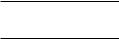
The solution is now complete, the flow rate being given by Eq. 4.4.15 and the arbitrary constants are given by Eqs.4.4.9,18,19. A plot of q(t) for a value of (4tL/tC ) < 1 where overdamping conditions prevail is shown in Fig. 4.4.1. Typically, the flow rate starts from a prescribed normalized value of 1.0 then gradually enters a phase of regular oscillations about a zero mean, consistent with the driving oscillatory pressure drop. These two phases in the dynamics of the RLC system will be discussed at great length in subsequent sections. Here we note only that the pattern of dynamics observed in Fig. 4.4.1 is analogous to the pattern observed in Fig. 3.3.1 for the overdamped case in free dynamics where the flow also starts from a prescribed normalized value of 1.0, then gradually diminishes to zero. The di erence between the two cases is only in the forced oscillations imposed in the present case.

Thus, the study of free dynamics of the RLC system in Section 3.3, though at first seemed somewhat artificial as a model of the physiological system, is now seen as an important integral part of an overall study of the system. We now see that the properties of the RLC system observed in free dynamics under the three di erent damping conditions are in fact intrinsic properties of the system that are equally relevant in forced dynamics.

Finally, we see now that in the general solution of the forced dynamics problem, broadly speaking, the homogeneous part of the solution, namely

The homogeneous part of the solution, qh(t), comes from the general solution of the free dynamics equation under the underdamped scenario and is given by (Eq. 3.3.14)

where A,B, are arbitrary constants.

The complete solution is then given by

As in the previous section, to find the arbitrary constants A, B, di erentiating this expression and evaluating at time t = 0 gives

Again, we note the reduced amount of algebra involved in this process because of the use of the complex exponential function.

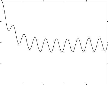
Results are shown in Fig. 4.5.1 for a value of (4tL/tC ) > 1.0 where underdamped conditions prevail. The flow rate starts from a prescribed normalized value of 1.0, undergoes some large irregular oscillations, then gradually enters a phase of regular oscillations about a zero mean, consistent with the driving oscillatory pressure drop. This pattern is analogous to the pattern observed in Fig. 3.3.1 for the underdamped case in free dynamics where the flow also starts from a prescribed normalized value of 1.0, undergoes some large irregular oscillations, then gradually diminishes to zero.

We note that both in free and in forced dynamics, underdamped conditions occur when

124 4 Forced Dynamics of the RLC System

t / tL

Fig. 4.5.1. Flow rate q(t) in an RLC system in series and in forced dynamics, with an oscillatory driving pressure drop. System parameters are such that (4tL/tC ) = 40, therefore producing underdamped conditions.

compared with the overdamped case considered in the previous section where the quantity in brackets is less than 1.0. Thus, all else being equal, underdamped conditions correspond to lower values of C which in turn corresponds to an elastic balloon which is less elastic. Thus, the initial oscillations observed in the underdamped case result from the recoiling of a sti er balloon. A balloon that is more elastic would instead absorb the filling without recoiling, as observed in the overdamped case.

4.6 Critically Damped Forced Dynamics

Between the overdamped and underdamped conditions, which occur over a range of values of 4tL/tC below and above 1.0, there is a singular condition corresponding to a single value of this ratio, namely

whereby the flow rate in the RLC system in series under conditions of forced dynamics moves “most directly” from its prescribed initial value to the state of forced oscillations being imposed on it. This is the scenario of critically damped forced dynamics, analogous to that of critical damping encountered in free dynamics.

As in the previous two sections, the flow rate solution again consists of two parts:

where the particular part of the solution, qp(t), is the same as before (Eq. 4.4.9), namely

The homogeneous part of the solution, qh(t), comes from the general solution of the free dynamics equation under the critically damped scenario and is given by (Eq. 3.3.17,16)

where A,B, are arbitrary constants. The complete solution is given by

and, to find the constants A, B, di erentiating this expression and evaluating at time t = 0 gives

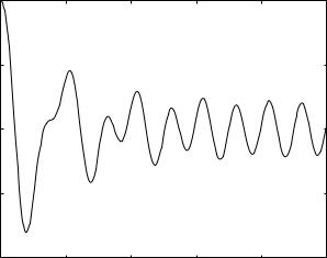
Results are shown in Fig. 4.6.1 for the value of (4tL/tC ) = 1.0 where critically damped conditions occur. The flow rate starts from a prescribed normalized value of 1.0, then gradually enters a phase of regular oscillations about a zero mean, consistent with the driving oscillatory pressure drop. This pattern is analogous to the pattern observed in Fig. 3.3.1 for the critically damped case in free dynamics where the flow also starts from a prescribed normalized value of 1.0, then gradually diminishes to zero. Both in free and in forced dynamics, the di erence between the overdamped and critically damped dynamics is one of degree only. In the critically damped case the flow rate moves towards its ultimate oscillations more “expediently” than it does in the overdamped case.

126 4 Forced Dynamics of the RLC System

t / tL

Fig. 4.6.1. Flow rate q(t) in an RLC system in series and in forced dynamics, with an oscillatory driving pressure drop. System parameters are such that (4tL/tC ) = 1.0, therefore producing critically damped conditions.

4.7 Transient and Steady States

Both in free and in forced dynamics the RLC system undergoes two distinct phases (Figs. 3.3.1, 4.4.1, 4.5.1, 4.6.1). In the first, which is widely referred to as the “transient state”, the system is adjusting to the imposed initial flow conditions and the flow rate continues to change accordingly. In the second, referred to as “steady state”, the adjustment is complete and no further change in the pattern of flow rate takes place.

We saw that in free dynamics the steady state is a state of zero flow because there is no imposed pressure drop to drive the flow. Any flow within the system is there because of the prescribed initial flow conditions. The transient state takes the system from these initial conditions to the steady state. Thus, the steady state may be viewed as that appropriate for the system under the particular driving force being imposed on it externally. In the absence of such forces, as in the case of free dynamics, the appropriate state is that of zero flow.

Similarly, in forced dynamics the steady state of the system is that appropriate for the applied external driving force. When the latter is oscillatory, as we saw in previous sections, the steady state of the system is that in which the flow rate oscillates in tandem with the externally imposed pressure drop. Again, the transient state takes the system from whatever initial conditions are prescribed to this steady state.

In analytical terms, the steady state of the RLC system is a particular solution of the governing equation (Eq. 3.2.5)

while the transient state of the system is a general solution of the reduced equation

In free dynamics the pressure drop is zero, therefore the term on the righthand side of Eq. 4.7.1 is zero and the equation becomes identical with Eq. 4.7.2. Therefore, in this case the steady state is a particular solution of Eq. 4.7.2 and the transient state is a general solution of the same equation. The general solution was obtained in Section 3.3 under the three di erent scenarios of overdamped, underdamped, and critically damped conditions. A particular solution of Eq. 4.7.2 is clearly q = 0, which is consistent with results in Section 3.3 indicating that the steady state of the system is that of zero flow under all three damping scenarios.

In forced dynamics the steady state of the RLC system depends on the form of the driving pressure drop Δp since this determines the form of the particular solution of Eq. 4.7.1. We saw that when the driving pressure drop is an oscillatory function of the form Δp(t) = Δp0eiωt where Δp0 is a constant, the particular solution is of the same form, namely q(t) = Keiωt where K is a constant. Thus, the steady state of the system is one in which the flow rate oscillates with the same frequency as the pressure drop. It is appropriate to refer to this as “steady state” even though the flow rate is a function of time. The term “steady” here is not to be confused with “constant”, it merely implies that the pattern of flow rate as a function of time is no longer changing.

The most important property of the transient state is that it occupies only a relatively short time from the onset of the initial flow conditions, then leaving the system in steady state thereafter. We saw that both in free and in forced dynamics, and under all three damping scenarios, the transient part of the flow rate, namely qh(t), vanishes soon after the initial flow onset, leaving the system with only the steady part of the flow, namely with qp(t). These results are illustrated graphically in Figs.4.7.1-4. Because of this, many studies find it appropriate to ignore the transient state dynamics of the RLC system and focus on the steady state dynamics only (see Chapter 7).

The relevance of this discussion to coronary blood flow is that practically all lumped model studies of the coronary circulation are based on only the steady state dynamics of the system.

One might attempt to examine the validity of this practice by noting from Fig. 4.7.1 that in free dynamics the RLC system comes very close to steady state when t/tL ≈ 15. In forced dynamics, results in Figs.4.7.2-4 indicate that