

suai.ru/our-contacts |
quantum machine learning |
Weights in CQQL |
137 |
Since our language obeys the rules of a Boolean algebra we can transform every possible CQQL condition into the required syntactical form, e.g., the disjunctive normal form or the one-occurrence-form [8]. Schmitt [2] gives an algorithm performing this transformation.
Our example condition without weights is a CQQL condition being already in the required form. Following DeÞnition 7 we obtain svT (o) · svA(o) · (svD (o) + svS (o) − svD (o) · svS (o))(1 − svP (o)) for an object o to be evaluated.
5 Logic-Based Weighting
Our approach of weighting CQQL conditions is surprisingly simple. The idea is to transform a weighted conjunction or a weighted disjunction into a logical formula without weights:
|
w (ϕ1 |
,ϕ2) |
(ϕ1 |
¬ |
θ1) |
|
(ϕ2 |
¬ |
θ2) |
and |
w (ϕ1,ϕ2) |
(ϕ1 |
|
θ1) |
|
(ϕ2 |
|
θ2). |
|
|
θ1,θ2 |
# |
|
|
|
|
|
θ1,θ2 |
# |
|
|
|
|
||||||
Definition 8 |
Let o be a database object, svac(o) [0, 1] a score value obtained |
||||||||||||||||||
from evaluating an atomic CQQL condition ac on o, Θ = {θ1, . . . , θn} with θi [0, 1] a set of weights, and ϕ a CQQL condition constructed by recursively applying, , θi ,θj , θi ,θj , and ¬ on a commuting set of atomic conditions. The weighted score function is deÞned by
f Θ |
|
|
(o) |
(ϕ1¬θi ) (ϕ2¬θj ) |
|
||
f Θ |
|
(o) |
|
(ϕ1 θi ) (ϕ2 θj ) |
|
|
|
"CQQL |
fϕΘ1 (o), fϕΘ2 (o) |
||
fϕΘ (o) = CQQL |
fϕΘ1 (o), fϕΘ2 (o) |
||
1 − fϕΘ1 (o) svac(o) svacθ
if ϕ = ϕ1 θi ,θj ϕ2
if ϕ = ϕ1 θi ,θj ϕ2
if ϕ = ϕ1 ϕ2 if ϕ = ϕ1 ϕ2 if ϕ = ¬ϕ1
if ϕ = ac if ϕ = θ.
svacθ can be regarded as a special atomic condition without argument returning the constant θ .
Our weighting does not require a special weighting formula outside of the context of logic. Instead it uses exclusively the power of the underlying logic. Please notice that we can weight not only atomic conditions but also complex logical expressions. Thus, our approach supports a nested weighting.
Figure 3 (left) shows the result of applying our mapping rules onto the weighted tree from Fig. 1. Following our CQQL evaluation we obtain the formula
suai.ru/our-contacts |
quantum machine learning |
138 |
|
|
|
|
|
|
|
|
|
|
I. Schmitt |
|
|
|
|
|
|
|
|
|
|
|
|
|
|
|
|
|
|
|
|
|
|
|
|
|
|
|
|
|
|
|
|
|
name |
θD |
θS |
θDS |
θP |
winner |
|
T A |
|
|
|
|
|
equi weight |
1 |
1 |
1 |
1 |
fair |
|
|
|
|
nonrelevant price |
1 |
1 |
1 |
0.1 |
deluxe |
|
|||
|
¬ |
¬ |
|
¬ |
|
|
||||||
|
P |
θP |
very relevant price |
1 |
1 |
0 |
1 |
cheap |
|
|||
|
|
θDS |
|
|
||||||||
|
|
|
|
|
|
very relevant date |
1 |
0.4 |
1 |
0.2 |
exact date |
|
|
|
|
|
zero weight |
0 |
0 |
0 |
0 |
cheap |
|
||
|
|
|
|
|
|
|
||||||
D θD S |
θS |
|
|
|
|
|
|
|
|
|
|
|
Fig. 3 Expanded weighted condition tree and weight settings
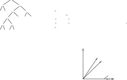
Fig. 4 Weight mapping for θ = 1/4 and θ = 1/2
|1 |
w = π/3 for θ = 1/4 |
w = π/4 for θ = 1/2 |
vector for constant 1 |
1 |0 |
fϕΘ (o) = svT (o) · svA(o) · svDSθ (o) · sv¬P θP (o)
svDSθ (o) = svDS (o) + (1 − svθDS ) − svDS (o) · (1 − svθDS )
svDS (o) = svD (o) · svθD + svS (o) · svθS − svD (o) · svθD · svS (o) · svθS sv¬P θP (o) = (1 − svP (o)) + (1 − svθP ) − (1 − svP (o)) · (1 − svθP ).
The table in Fig. 3 (right) shows the chosen weight values and the corresponding cottages with the highest score value. Of course, for an end user it is not easy to Þnd the right weight values. Instead, we propose the usage of linguistic variables like very important, important, neutral, less important, and not important and map them to numerical weight values. Another possibility is to use graphical weight sliders to adjust the importance of a condition.
Next, we show that our weighting approach fulÞlls our requirements.
Theorem 2 The weight functions as defined in Definition 8 fulfill the requirements R1 to R5.
Proof Following Theorem 1, CQQL conditions with conjunction, disjunction, and negations form a Boolean algebra. Our approach uses special atomic conditions acθ for different weights θ (Fig. 4).
As demonstrated, our weighting is realized inside the CQQL logic. Thus, it is easy to show the fulÞllment of the requirements:
1.(R1) weight=0: w0",1(a, b) = (a ¬0) (b ¬1) = 1 b = b. The commutative variant and the disjunction are analogously fulÞlled.

suai.ru/our-contacts |
quantum machine learning |
Weights in CQQL |
139 |
2.(R2) weight=1: w1",1(a, b) = (a ¬1) (b ¬1) = a b = "CQQL(a, b)
(analogously for ).
3.(R3) continuity: The weight functions are continuous on the weights since the underlying squared cosine function, conjunction, and disjunction are continuous.
4.(R4) embedding in a logic: Since our weighting is realized inside the logic formalism the resulting logic is still a Boolean algebra. The proof of the four formulas is thus straightforward.
5.(R5) linearity: The evaluation of a weighted CQQL conjunction and disjunction w.r.t. one weight is based on linear formulas.
So far, we applied our weighting approach to retrieval and proximity conditions of our CQQL language. What about applying it exclusively to traditional database conditions returning just Boolean values? In that case, we distinguish between two cases:
1.Non-Boolean weights: If the weights come from the interval [0, 1], then we
cannot use the normal Boolean disjunction and conjunction. Instead we propose to replace them with the algebraic sum (x + y − x · y) and the algebraic product (x · y). This case can be regarded as a special case (only database conditions) of CQQL and it fulÞlls the requirements (R1) to (R5) if each condition is not weighted more than once. Otherwise we transform, see [2], that formula into
the required form. Table 2 shows the effect of non-Boolean weights on database conditions whose evaluations are expressed by x and y.
2. Boolean weights: If the weights are Boolean values, then we can evaluate a weighted formula by using Boolean conjunction and disjunction fulÞlling requirements (R1), (R2), and (R4). Requiring continuity (R3) and linearity (R5) on Boolean weights is meaningless. Boolean weights have the effect of a switch. A weighted condition can be switched to be active or inactive.
At the end, we present (x θ ) (y ¬θ ) as an interesting special case where one connected weight instead of two weights is used. In this case, the resulting evaluation formula is the weighted sum: θ svx (o) + (1 − θ ) svy (o). Very surprisingly, next logical transformation3 shows that connected weights of a conjunction equal exactly connected weights of a disjunction.
Table 2 Weights on Boolean conditions
x |
|
y |
|
|
x θ,1 y := x + |
|
|
|
|
x θ,1 y := θ x + y − θ xy |
||
|
|
θ |
− xθ |
y |
||||||||
0 |
(false) |
0 |
(false) |
0 |
(false) |
0 |
(false) |
|||||
0 |
(false) |
1 |
(true) |
|
|
|
|
|
|
|
1 |
(true) |
|
θ |
|
|
|
|
|
||||||
1 |
(true) |
0 |
(false) |
0 |
(false) |
θ |
|
|||||
1 |
(true) |
1 |
(true) |
1 |
(true) |
1 |
(true) |
|||||
3For a simple notation, conjunction is expressed by a multiplication and disjunction by an addition symbol.

suai.ru/our-contacts |
quantum machine learning |
140
Fig. 5 Connected weights between conjunction and disjunction
|
|
I. Schmitt |
1 |
|
0.5 y = 0.5 + y − 0.5 y |
|
|
|
|
|
0.5 0,1 y = y |
0.5 |
|
0.5 0.5,0.5 y = 0.25 + 0.5 y |
|
|
0.5 1,0 y = 0.5 |
|
|
0.5 y = 0.5 y |
0 |
1 |
y |
|
(x + ¬θ )(y + θ ) = xy + xθ + y¬θ + ¬θ θ = xyθ + xy¬θ + xθ + y¬θ
= (xy + x)θ + (xy + y)¬θ = xθ + y¬θ.
This effect can be interpreted as a neutral combination of conditions. Figure 5 illustrates for a constant x = 0.5 that x θ,1−θ y lies exactly in the middle between conjunction and disjunction.
6 Related Work
Weighting of non-Boolean query conditions is a well-known problem. Following [9], we distinguish four types of weight semantics: (1) weight as measure of importance of conditions, (2) weight as a limit on the amount of objects to be returned, (3) weight as threshold value, cf. [10, 11], and (4) weight as speciÞcation of an ideal database object. Next, we discuss related papers about weights as measure of importance. All logic-based weighting approaches supporting vagueness use the fuzzy t-norm/t-conorm min/max.4 In contrast, our approach is a general logicbased approach where min/max is just one special case.
Fagin’s Approach Fagin and Wimmers [4] propose a special arithmetic weighting formula to be applied on a score rule S. Let Θ = {θ1, . . . , θn} be weights with
θi |
[ |
0, 1 |
] |
|
i |
|
Θ= |
1, and θ1 |
≥ |
|
≥ |
|
≥ |
θn. The weighted version of the score is |
|
|
|
, |
|
θi |
|
|
θ2 |
|
. . . |
|
|||||
then deÞned as S |
|
(μ1(o), . . . , μn(o), θ1, . . . , θn) = (θ1−θ2)S(μ1(o))+2 (θ2−θ3) |
|||||||||||||
S(μ1(o), μ2(o))+. . .+n θnS(μ1(o), . . . , μn(o)). Since this weighting approach is on top of a logic it violates R4. Thus, associativity in combination with min/max, for example, cannot be guaranteed (see [12]). Furthermore, Sung [13] describes a so-called stability problem for FaginÕs approach. We can show that FaginÕs formula with weights θ1F , θ2F applied to our CQQL logic can be simulated by our weighting where θ1 = 1 and θ2 = 2 θ2F hold.
4min/max is the only fuzzy t-norm/t-conorm which supports idempotence and distributivity.