Fig. 1 Two main lines connecting abstract to concrete exist in the human culture. The Þrst one goes from concrete objects to more abstract collections of objects having common features. The second one goes from abstract single-word concepts to stories formed by the combination of many meaning-connected concepts

2 The Double-Slit Experiment

The double-slit experiment is among the paradigmatic quantum experiments and can be used to effectively illustrate the rationale of our quantum modeling of the meaning content of corpora of written documents. One of the best descriptions of this experiment can be found in FeynmanÕs celebrated lectures in physics [24]. We will provide three different descriptions of the experiment. The Þrst one is just about what can be observed in the laboratory, showing that an interpretation in terms of particle or wave behaviors cannot be consistently maintained. The second (Sect. 3) one is about characterizing the experiment in a conceptualistic way, attaching to the quantum entities a conceptual-like nature, and to the measuring apparatus a cognitive-like nature. The third one is about interpreting the experiment as an IRlike process (Sect. 4).

We Þrst consider the classical situation where the entities entering the apparatus, in its different conÞgurations, are small bullets. Imagine a machine gun shooting a stream of these bullets over a fairly large angular spread. In front of it there is a barrier with two slits (that can be opened or closed), just about big enough to let a bullet through. Beyond the barrier, there is a screen stopping the bullets, absorbing them each time they hit it. Since when this happens a localized and visible trace of the impact is left on the screen, the latter functions as a detection instrument, measuring the position of the bullet at the moment of its absorption. Considering that the slits can be opened and closed, the experiment of shooting the bullet and observing the resulting impacts on the detection screen can be performed in four different conÞgurations. The Þrst one, not particularly interesting, is when both slits

Fig. 2 A schematic description of the classical double-slit experiment, when: (A) only the left slit is open; (B) only the right slit is open; and (AB) both slits are simultaneously open. Note that the time during which the machine gun Þred the bullets in situation (AB) is twice than in situations

(A) and (B)

are closed. Then, there are no impacts on the detection screen, as no bullets can pass through the barrier. On the other hand, impacts on the detection screen will be observed if (A) the left slit is open and the right one is closed; (B) the right slit is open and the left one is closed; (AB) both slits are open. The distribution of impacts observed in these three conÞgurations is schematically depicted in Fig. 2. As one would expect, the Ôboth slits openÕ situation can be easily deduced from the two Ôonly one-slit openÕ situations, in the sense that if μA(x) and μB (x) are the probabilities of having an impact at location x on the detection screen, when only the left (resp., the right) slit is open, then the probability μAB (x) of having an impact at that same location x, when both slits are kept open, is simply given by the uniform average:

Consider now a similar experiment, using electrons instead of small bullets. As well as for the bullets, well-localized traces of impact are observed on the detection screen in the situations when only one slit is open at a time, always with the traces of impact distributed in positions that are in proximity of the open slit. On the other hand, as schematically depicted in Fig. 3, when both slits are jointly open, what is obtained is not anymore deducible from the two Ôonly one-slit openÕ situations. More precisely, when bullets are replaced by electrons, (1) is not anymore valid and we have instead:

where IntAB (x) is a so-called interference contribution, which corrects the classical uniform average (1) and can take both positive and negative values. Clearly, a corpuscular interpretation of the experiment becomes now impossible, as the region

Fig. 3 A schematic description of the quantum double-slit experiment, when: (A) only the left slit is open; (B) only the right slit is open; and (AB) both slits are simultaneously open. Different from the classical (corpuscular) situation, a fringe (interference) pattern appears when the left and right slits are both open

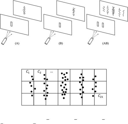
Fig. 4 The detection screen, partitioned into n = 21 different cells, each one playing the role of an individual position detector, here showing the traces of m = 54 impacts. The experimental

probabilities are: μAB (C1; 21) = 542 , μAB (C2; 21) = 542 , μAB (C3; 21) = 541 , μAB (C4; 21) = 547 ,. . . , μAB (C20; 21) = 541 , μAB (C21; 21) = 0

where most of the traces of impact are observed is exactly in between the two slits, where instead we would expect to have almost no impacts. Also, in the regions in front of the two slits, where we would expect to have the majority of impacts, practically no traces of impact are observed.

Imagine for a moment that we are only interested in modeling the data of the experiment (either with bullets or electrons) in a very instrumentalistic way, by limiting the description only to what can be observed at the level of the detection screen, i.e., the traces that are left on it. For this, one can proceed as follows. The surface of the detection screen is Þrst partitioned into a given number n of numbered cells C1, . . . , Cn (see Fig. 4). Then, the experiment is run until m traces are obtained on it, m being typically a large number. Also, the number of traces of impact in each cell is counted. If mAB (Ci ) is the number of traces counted in cell Ci , i = 1, . . . , n, the experimental probability of having an impact in that cell is given by the ratio

mAB (Ci ) . Here by Ôexperimental probabilityÕ we simply mean the

m

probability ÒinducedÓ by a relative frequency over a large number of repetitions of a same measurement, under the same experimental conditions. Similarly, we have

the number of traces counted in cell Ci when only the left and right slits are kept open, respectively. If the experiments are performed using small bullets, one Þnds that the difference μAB (Ci ; m) − 12 [μA(Ci ; m) + μB (Ci ; m)] tends to zero, as m tends to inÞnity, for all i = 1, . . . , n, whereas if the experiment is done using microentities, like electrons, it does not converge to zero, but towards a function Int(Ci ), expressing the amount of deviation from the uniform average situation.

Now, once the three real functions μA(Ci ; m), μB (Ci ; m), and μAB (Ci ; m) have been obtained, and their m → ∞ limit deduced, one could say to have successfully modeled the experimental data, in the three different conÞgurations of the barrier. However, a physicist would not be satisÞed with such a modeling. Why? Well, because it is not able to explain why μAB (Ci ) = limm→∞ μAB (Ci ; m) cannot be deduced, as one would expect, from μA(Ci ) = limm→∞ μA(Ci ; m) and μB (Ci ) = limm→∞ μB (Ci ; m), and why μAB (Ci ) possesses such a particular interference-like fringe structure. So, let us explain how the quantum explanation typically goes. For this, we will need to exit the two-dimensional plane of the detection screen and describe things at a much more abstract and fundamental level of our physical reality.

As is well-known, even if our description extends from the two-dimensional plane of the detection screen to the three-dimensional theater containing the entire experimental apparatus, this will still be insufÞcient to explain how the interference pattern is obtained. Indeed, electrons cannot be modeled as spatial waves, as they leave well-localized traces of impact on a detection screen, and they cannot be modeled as particles, as they cannot be consistently associated with trajectories in space.3 They are truly Òsomething else,Ó which needs to be addressed in more abstract terms. And this is precisely what the quantum formalism is able to do, when describing physical entities in terms of the abstract notions of states, evolutions, measurements, properties, and probabilities, not necessarily attributable to a description of a spatial (or spatiotemporal) kind.

So, let |ψ be the state of an electron4 (at a given moment in time) after having interacted with the double-slit barrier, with both slits open (we use here DiracÕs notation). We can consider that this vector state has two components: one corresponding to the electron being reßected back towards the source (assuming for simplicity that the barrier cannot absorb it), and the other one corresponding to the electron having successfully passed through the barrier and reached the detection screen. Let then PC be the projection operator associated with the property of Òhaving been reßected back by the barrier,Ó and PAB the projection operator associated with the property of Òhaving passed through the two slits.Ó For instance,

3This statement remains correct even in the de BroglieÐBohm interpretation of quantum mechanics, as in the latter the trajectories of the micro-quantum entities can only be deÞned at the price of introducing an additional non-spatial Þeld, called the quantum potential.

4One should say, more precisely, that |ψAB is a Hilbert-space vector representation of the electron state, as a same state can admit different representations, depending on the adopted mathematical formalism.

10 D. Aerts et al.

PC could be chosen to be the projection onto the set of states localized in the halfspace deÞned by the barrier and containing the source, whereas PAB would project onto the set of states localized in the other half-space, containing the detection screen.5 We thus have PC + PAB = I, and we can deÞne |ψAB = , which is the state the electron is in after having passed through the barrier and reached the detection screen region. Note that the barrier acts as a Þlter, in the sense that if the electron does leave a trace on the detection screen, we know it did successfully pass through the barrier, and therefore was in state |ψAB when detected.

Now, since by assumption the n cells Ci of the detection screen work as distinct measuring apparatuses, and an electron cannot be simultaneously detected by two different cells, for all practical purposes we can associate them with n orthonormal vectors |ei , ei |ej = δij , corresponding to the different possible outcome-states of the position measurement performed by the screen. This means that we can consider {|e1 , . . . , |en } to form a basis of the subspace of states having passed through the barrier, and since we are not interested in electrons not reaching the detection screen, we can consider such n-dimensional subspace to be the effective Hilbert space H of our quantum system, which, for instance, can be taken to be isomorphic to the vector space Cn of all n-tuples of complex numbers.

According to the Born rule (which in quantum mechanics is used to obtain a correspondence between what is observed in measurement situations, in terms of relative frequencies, and the objects of its mathematical formalism, thus expressing the statistical content of the theory and allowing to bring the latter in contact with the experiments), the probability for an electron in state |ψAB H, to be detected by cell Ci , is given by the square modulus of the amplitude ei |ψAB , that is: μAB (Ci ) = | ei |ψAB |2, and if we assume that an electron that has passed through the barrier is necessarily absorbed by the screen (assuming, for instance, that the

projection operators Pi = |ei ei |, we can also write, equivalently:

μAB (Ci ) = Pi |ψAB 2 = ψAB |Pi Pi |ψAB = ψAB |Pi2|ψAB = ψAB |Pi |ψAB .

(3) More generally, if I is a given subset of {1, . . . , n}, we can deÞne the projection operator M = i I Pi , onto the set of states localized in the subset of cells with indexes in I , and the probability of being detected in one of these cells is given by:

5Intuitively, one can also think of PAB as the projection operator onto the set of states having their momentum oriented towards the detection screen. Of course, all these deÞnitions are only meaningful if applied to asymptotic states, viewing the interaction of the electron with the barrier as a scattering process, with the barrier playing the role of the local scattering potential.

impact to appear in the central vertical sector of the screen (the central fringe) is one-third.

The double-slit experiment does not allow to determine if an electron that leaves a trace of impact on the detection screen has passed through the left slit or the right slit. This means that the properties Òpassing through the left slitÓ and Òpassing through the right slitÓ remain potential properties during the experiment, i.e., alternatives that are not resolved and therefore (as we are going to see) can give rise to interference effects [24]. Let however write PAB as the sum of two projectors: PAB = PA + PB , where PA corresponds to the property of Òpassing through the left slitÓ and PB to the property of Òpassing through the right slit.Ó Note that there is no unique way to deÞne these properties, and the associated projections, as is clear that electrons are not corpuscles moving along spatial trajectories. A possibility here is to further partition the half-space deÞned by PAB into two sub-half-spaces, one incorporating the left slit, deÞned by PA and the other one incorporating the right slit, deÞned by PB , so that PAPB = PB PA = 0. For symmetry reasons, we can assume that the electron has no preferences regarding passing through the left or right slits (this will be the case if the source is placed symmetrically with respect to the two slits),

According to the above deÞnitions, |ψA and |ψB can be interpreted as the states describing an electron passing through the left and right slit, respectively.6 In other words, in accordance with the quantum mechanical superposition principle, we have expressed the electron state in the double-slit situation as a (uniform) superposition of one-slit states. Inserting (5) in (4), now omitting the argument in the brackets to simplify the notation, we thus obtain:

μAB = ψAB |M|ψAB = 1 ( ψA| + ψB |)M(|ψA + |ψB )

2

=1 ( ψA|M|ψA + ψB |M|ψB + ψA|M|ψB + ψB |M|ψA )

2

IntAB

6Note however that, as we mentioned already, it is not possible to unambiguously deÞne the two projection operators PA and PB , for instance, because of the well-known phenomenon of the spreading of the wave-packet. In other words, there are different ways to decompose |ψAB as the superposition of two states that can be conventionally associated with the one-slit situations, as per (5).