


 Revised: 21 January 2020
  Accepted: 4 February 2020
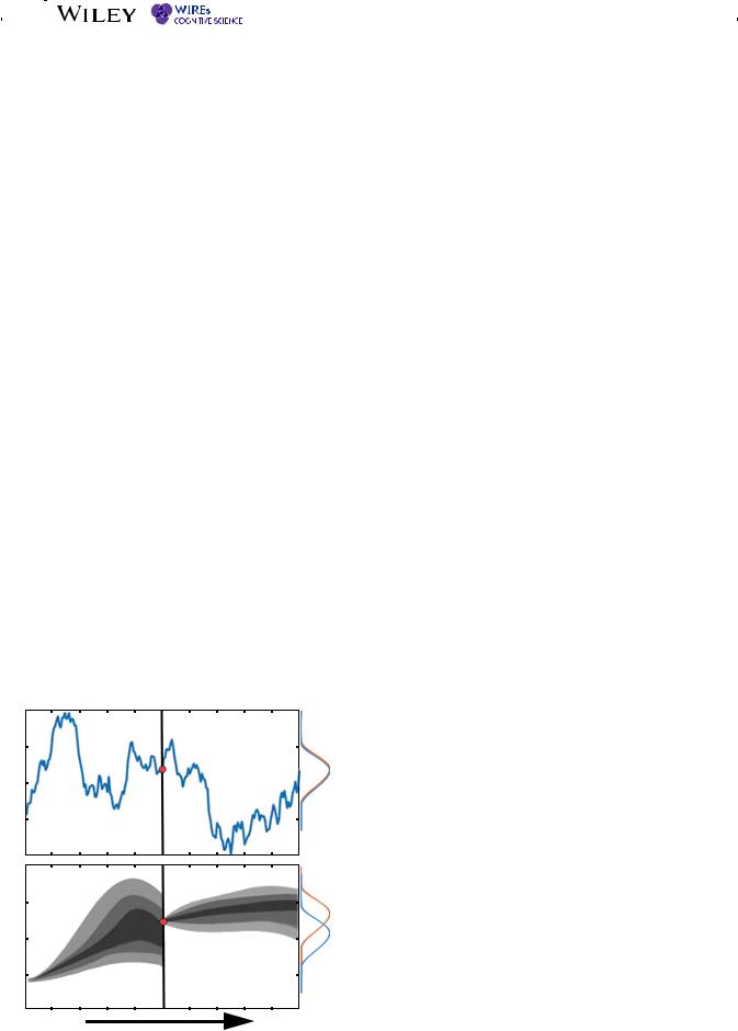

suai.ru/our4 |
|
- |
contacts |
|
|
quantum machine learning |
||
|
|
|
||||||
|
of 19 |
|
|
|
|
|
BUSEMEYER ET AL. |
|
|
|
|
|
|
|
|
|
|
different. On the one hand, the probabilities of Markov processes represent epistemic uncertainty, which is an observer's (e.g., a modeler's) lack of knowledge about the underlying true state existing at each moment in time due to a lack of information about the decision maker's beliefs. On the other hand, the amplitudes of quantum processes represent ontic uncertainty, which is the intrinsic uncertainty about the constructive result that a measurement generates at each moment in time (Atmanspacher, 2002). Ontic uncertainty cannot be reduced by greater knowledge about the decision maker's state.
These are two strikingly different views about the nature of change in belief during evidence accumulation. Markov processes, which include the popular random walk/diffusion models (Diederich & Busemeyer, 2003; Ratcliff et al., 2016), are more established, and have a longer history with many successful applications. These include both the simple random walk models, where a decision maker has a discrete set of states (e.g., 11 confidence levels, 0/10/20/…/100) that they move through over time, shown in Figure 2, and the more common diffusion models where the “states” are a continuously-valued level of evidence (such as 0–100, including all numbers in between). Since the discrete-state random walks approach a diffusion process as the number of states gets very large, we group these two approaches together under the umbrella of Markov process, which have been used to model choices and response times (Emerson, 1970; Luce, 1986; Stone, 1960) as well as probability judgments (Edwards, Lindman, & Savage, 1963; Kvam & Pleskac, 2016; Moran, Teodorescu, & Usher, 2015; Ratcliff & Starns, 2009; Wald & Wolfowitz, 1948; Wald & Wolfowitz, 1949; Yu, Pleskac, & Zeigenfuse, 2015) in domains such as memory (Ratcliff, 1978), categorization (Nosofsky & Palmeri, 1997), and inference (Pleskac & Busemeyer, 2010).
Although quantum processes have a long and successful history in physics, they have only recently been considered for application to human decision making (Busemeyer & Bruza, 2012; Khrennikov, 2010). However, a series of studies have aimed at testing and comparing these two competing views of evidence accumulation. The purpose of this article is to (a) provide an introduction to these two contrasting views, (b) review the research that directly tests and compares these types of theories, and (c) draw conclusions about conditions that determine when each view is more valid, or whether a mixture of the two processes might be needed for a more complete theory.
3 | BASIC PRINCIPLES OF MARKOV AND QUANTUM DYNAMICS
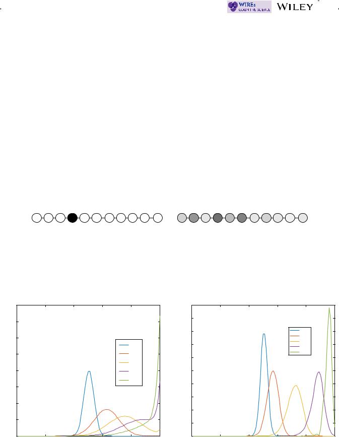
Although the introduction focused on evidence accumulation that occurs during inferential choice problems, Markov and quantum models are based on general principles that can be applied to both evidence and preference accumulation problems. Table 1 provides a side by side comparison of the five general principles upon which the two theories are based. Both theories begin with a set of possible basic states that the system can pass through over time, describing the relative degrees of support for one option or the other. In the case of evidence accumulation, these states are distinct levels of belief. Figure 2 uses 11 levels, but actual applications typically use a much larger number so as to approximate a continuum. In the case of preference accumulation, these states are distinct levels of preference.
State representation principle: For the Markov model, there is a probability distribution across states at each point in time. The probability assigned to each basic state conceptually represents the likelihood that an outside observer might attribute to the decision maker being located at that state. This probability distribution always sums to one. For the quantum model, there is an amplitude distribution across states at each point in time. The amplitude assigned to a basic state can be a real or complex number, and the probability of reporting that state is the squared magnitude of the amplitude.1 The sum of squared amplitudes always sums to one (i.e., the amplitude distribution has unit length). The nonlinear map from amplitudes to probabilities is an important way the two theories differ, and as we will see in the next section on an interference effect, it leads to testable competing predictions.
Principle |
Markov |
Quantum |
|
|
T A B L E 1 Five basic principles |
|
|
underlying Markov and quantum |
|||
1: State representation |
Probability distribution |
Amplitude distribution |
|
|
|
|
|
dynamics |
|||
|
|
|
|
|
|
2: State evolution |
Transition operator |
Unitary operator |
|
|
|
3: Rate of change |
Kolmogorov equation |
Schrödinger eqaution |
|
|
|
|
|
|
|
|
|
4: Dynamic operators |
Intensity operator |
Hamiltonian operator |
|
|
|
5: Response selection |
Measurement operator |
Measurement operator |
|
|
|
|
|
|
|
|
|

suai.ru/our-contacts |
quantum |
machine |
|
learning |
||||
|
||||||||
|
BUSEMEYER ET AL. |
|
|
|
|
|
5 of 19 |
|
State evolution principle: For the Markov model, the probability distribution over states evolves for period of time t > 0 according to a linear transition operator. This operator describes the probability of transiting from one basic state to another over some period of time t, representing how incoming information changes the probability distribution over states across time. For the quantum model, the amplitude distribution evolves for a period of time t > 0 according to a linear unitary operator. This operator describes the amplitude for transiting from one basic state to another over some period of time t. Once again, the probability of making this transition is obtained from the squared magnitude. In other applications, the unitary operator can also specify how the state changes according to some fixed amount of new information, such as a single vignette (Trueblood & Busemeyer, 2011) or cue in the choice environment (Busemeyer, Pothos, Franco, & Trueblood, 2011). The unitary operator is required to maintain a unit length amplitude distribution over states across time, thus constraining the sum of squared amplitudes representing the probability of observing different measurement outcome to be equal to one.
Rate of change principle: For the Markov model, the rate of change in the probability distribution is determined by a linear differential equation called the Kolmogorov equation. The integration of these momentary changes are required to form a transition operator. For the quantum model, the rate of change in the amplitude distribution is determined by the Schrödinger equation. The integration of these momentary changes are required to form a unitary operator. These two linear differential equations are not shown here, but they are strikingly similar, except for the complex number i that appears in the Schrödinger equation (which is the reason for using complex amplitudes).
For the Markov model, the linear differential equation is defined by an intensity operator that contains two key parameters: a “drift rate” parameter that determines the direction of change and a “diffusion” parameter that determines the dispersion of the probability distributions. The intensity operator of the Markov model has to satisfy certain properties to guarantee that the linear differential equation produces a transition operator. For the quantum model, the linear differential equation is defined by a Hamiltonian operator that also contains two key parameters: a parameter that determines the “potential function” which controls the direction of change and a “diffusion” parameter that determines the dispersion of the amplitude distribution. The Hamiltonian operator of the quantum model has to satisfy different properties than the intensity operator to guarantee that the linear differential equation produces a unitary operator, but it serves a similar function by evolving the corresponding state according to incoming information. These operators are the key ingredients of any stochastic processing theory and they contain the most important parameters for building a model.
Response selection: For the Markov model, the probability of reporting a response at some point in time equals the sum of the probabilities over the states that map into that response. After observing a response, a new probability distribution, conditioned on the observed response, is formed for future evolution. This probability distribution represents the updated information of an outside observer, where the measurement has reduced their uncertainty about the decision-maker's state. For the quantum model, the probability of reporting a response at some point in time equals the sum of the squared amplitudes over the states that map into that response. After observing a response, a new amplitude distribution, conditioned on the observed response, is formed for future evolution. In quantum models, this conditioning on the observed response is sometimes called the “collapse” of the wave function, which represents a reduction in the ontic uncertainty about the decision maker's evidence level, informing both the decision maker and an outside observer about the decision maker's cognitive state.
Despite the apparent similarities between the quantum and Markov processes outlined in the table, the two processes produce quite distinct behavior. For example, consider two processes shown in Figure 3 again. The Markov process in this figure is analogous to a pile of sand with wind blowing the sand to the right, where the sand eventually piles up in an equilibrium distribution. The quantum process in this figure is more closely analogous to a wave of water with the wind blowing the wave to the right. Once the wave hits the right wall, it bounces back until the wind blows it forward again. The result is that the quantum model does not reach an equilibrium, and instead it oscillates back and forth to the right across time. This interesting behavior is examined later in this article when we discuss preferential evolution. The following sections review previous applications of these models to evidence accumulation problems like choice, confidence, and response time, followed by applications to preference evolution.

suai.ru/our6 |
|
- |
contacts |
|
|
quantum machine learning |
||
|
|
|
||||||
|
of 19 |
|
|
|
|
|
BUSEMEYER ET AL. |
|
|
|
|
|
|
|
|
|
|
4 | INTERFERENCE EFFECTS
The state representation and the response selection process in the Markov process relies on a property that we call the read-out assumption. In Markov models, a judgment or a decision is made by mapping an existing state of evidence onto a response. For instance, a choice is made when evidence reaches a predetermined level of evidence, triggering the appropriate response. Other responses are modeled similarly as a read-out from an existing level of evidence: confidence, for instance, is typically modeled by mapping predetermined levels of evidence to confidence ratings (Moran et al., 2015; Pleskac & Busemeyer, 2010; Ratcliff & Starns, 2009), as are preference ratings (Bhatia & Pleskac, 2019) and judgments like willingness to pay, willingness to accept, and certainty equivalent prices (Johnson & Busemeyer, 2005; Kvam & Busemeyer, 2019).
This read-out assumption bears a striking resemblance to the assumption in economic models that preferences and beliefs are revealed by the choices people make (McFadden, Machina, & Baron, 1999; Samuelson, 1938). Yet decades of research from judgment and decision making and behavioral economics suggests that preferences are not revealed by the choices people make, but rather constructed by the process of generating a response like a choice (Ariely & Norton, 2008; Lichtenstein & Slovic, 2006; Payne, Bettman, & Johnson, 1992; Slovic, 1995). This construction of preference is typically understood as the result of people selecting a specific procedure from a larger repertoire of possible strategies to formulate a response (Gigerenzer et al., 1999; Hertwig et al., 2019; Payne, Bettman, & Johnson, 1993; Tversky, Sattath, & Slovic, 1988), or the dynamic nature of information accumulation that adjusts preferences over time (Busemeyer & Townsend, 1993; Johnson & Busemeyer, 2005). But quantum models, which model a judgment or decision as a measurement process that creates or constructs a definite state from an indefinite (superposition) state, offer a potentially more apt account of this hypothesis that preferences and beliefs are constructed.
5 | INTERFERENCE EFFECTS OF CHOICE ON CONFIDENCE
What are the behavioral implications of this process of constructing a definite state from an indefinite state? If information processing stops after the choice or judgment, then behaviorally this process is hard to dissociate from the classical read-out assumption of Markov models. However, if processing continues after a choice is made, then the two theories can make very different predictions about subsequent judgments. For instance, consider the situation when people are asked to make a choice and then rate their confidence in their choice—such paradigms are common in studies designed to study metacognition and confidence (Lichtenstein, Fischhoff, & Phillips, 1982; Yeung & Summerfield, 2012). If we model evidence accumulation during this situation as a Markov process, then a choice is a read-out of the location of the evidence, and the subsequent confidence judgment is just another read-out. However, we also know that in general evidence accumulation does not stop after the choice and that people continue to collect evidence after their choice (Baranski & Petrusic, 1998; Moran et al., 2015; Pleskac & Busemeyer, 2010; Yu et al., 2015). Consequently, a confidence judgment is made based on the evidence accumulated to make a choice as well as the evidence from postdecisional processing. Because classical models of evidence accumulation do not change the state of the evidence when it is measured, making a choice does not have an impact on the confidence people report. Thus, if a choice is made, but we ignore the choice, then the confidence should be the same as if they made no choice at all. In comparison, in a quantum process, a choice does changes the state of the evidence when a choice is made, and so even if we ignore the choice, the simple act of measurement does impact confidence judgments following subsequent evidence accumulation.
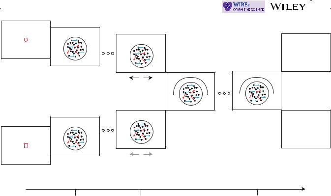
These are parameter-free competing predictions that hold for a large range of evidence accumulation processes, including ones where there is decay and trial-by-trial variability (for a mathematical proof, see Kvam et al., 2015). In general, they arise from the first-principles of each of the theories. To get an intuitive feel for the predictions, consider the experiment shown in Figure 4 that Kvam et al. (2015) asked participants to complete. In the experiment, participants viewed a random dot motion stimulus where a percentage of the dots moved coherently in one direction (left or right), and the rest moved randomly. In half of the blocks of trials participants were prompted at time point t1 (0.5 s) to decide whether the coherently moving dots were moving left or right and entered their choice via a mouse. In the the other half of the blocks—the no-choice condition—participants were prompted at t1 to click a predetermined mouse button. In all the trials, at a second time point t2, participants were prompted to rate their confidence that the coherently moving dots were moving right ranging from 0% (certain left) to 100% (certain right).
The prediction of no interference from the Markov model arises because it models evidence accumulation as the evolution of the probability distribution over evidence levels across time. In the choice condition, according to the

suai.ru/our-contacts |
quantum |
machine |
|
learning |
||||
|
||||||||
|
BUSEMEYER ET AL. |
|
|
|
|
|
9 of 19 |
|
time points, whereas the quantum model predicted an interference effect of the first rating on the second. The effects were more subtle—the results produced significant differences only for the lowest coherence levels, and were present at the individual level for only 3 out of the 11 participants at the low (2, 4%) coherence levels. Thus, the the results suggest that interference effects do occur with sequences of judgments, but they are small and occur for only a subset of the participants and coherence conditions. One way to interpret this difference in empirical results is that using a binary decision for the first measurement may be more effective for producing a “collapse” as compared to making a probabilistic judgment, potentially suggesting that different types of measurements may have different effects on the evidence state.
This experiment also made it possible for a generalization test (Busemeyer & Wang, 2000) to quantitatively compare the Markov and quantum models. Unlike the Bayes factor method previously used by Kvam et al. (2015), the generalization test provides a method to test a priori predictions of the models in new conditions. To do this, the parameters of the models were estimated using results obtained from conditions 1 and 2 for each individual; and then these same parameters were used to predict probability ratings for each person on the third condition (see Figure 5). For 8 of the 11 participants the comparison favored the quantum model for coherence levels 2, 4, and 8%, but only 5 participants produced results favoring the quantum model for coherence level 16%. The results clearly favored the quantum model overall, but less so for high coherence. These results indicated that some features of both Markov and quantum models may be needed to accurately account for the results. The quantum model seems to perform better at the low coherence levels and the Markov model begins to do better at the higher coherence levels.
7 | CATEGORIZATION-DECISION PARADIGM
Of course, choice and confidence judgments about dot motion direction are not the only situations in which people may be tasked with making multiple responses in sequence. Another illustration of the effects of sequential responses comes from a paradigm where participants were asked to make a category judgment about a face shown on the screen and a decision about how to interact with that face (Townsend, Silva, Spencer-Smith, & Wenger, 2000). In this study, the faces shown on screen could belong to one of two groups: a hostile group and a friendly group. The categorization judgment, when prompted, asked participants to determine which group the face belonged based on the relative width of the face (e.g., wider faces were more likely to be friendly and narrower faces more likely to be hostile). The decision component of the task regarded how to interact with that face: to act defensively or to act friendly. The optimal behavior was to act defensively in response to hostile / narrow faces, and act friendly with friendly / wide faces.
The key manipulation in this study was whether or not the defensive/friendly decision was preceded by a categorization judgment, or whether the decision was made alone (and similarly, whether the categorization judgment would be affected if it were preceded by an action decision). It was designed to test the Markov assumption that the marginal probabilities of acting defensive/friendly should not depend on whether or not there was a categorization judgment preceding it. Although the time course of these responses was not precisely controlled as in the interference studies above, the result similarly violated the law of total probability. Participants were more likely to act defensively when the decision was presented alone (without the categorization beforehand) than when it was preceded by the additional response (Busemeyer et al., 2009a; Wang & Busemeyer, 2016b). Conversely, Busemeyer, Wang, and Lambert-Mogiliansky (2009b) developed a quantum model that was permitted to violate the law of total probability, but constrained to obey another law called double stochasticity. Participants' decisions more closely followed the predictions of the quantum model by violating the law of total probability without violating the law of double stochasticity. This constitutes another domain in which interference between a sequence of responses generates a pattern of results in direct conflict with predictions of a Markov model.
Similar quantum models have been used to explain findings such as the disjunction effect in the Prisoner's dilemma (Pothos & Busemeyer, 2009; Tversky & Shafir, 1992) and two-stage gambling paradigms (Busemeyer, Wang, & Shiffrin, 2015; Shafir & Tversky, 1992), and other measurement effects on preference (Sharot, Velasquez, & Dolan, 2010; White, Barqué-Duran, & Pothos, 2016; White, Pothos, & Busemeyer, 2014). However, these experiments do not examine the time at which responses are made and the corresponding models tend to have simpler nondynamical structures, so they are not reviewed here.

suai.ru/our |
|
- |
contacts |
|
|
quantum machine learning |
||
|
|
|
||||||
|
10 of 19 |
|
|
|
|
|
BUSEMEYER ET AL. |
|
|
|
|
|
|
|
|
|
|
8 | SUMMARY
Taken together, these experiments help us hone in on the conditions in which the evidence accumulation may best be described as a quantum process and why. First, as we have established, based on first-principles, the Markov models predict that earlier responses do not impact the evidence accumulation process that helps determine later responses. Yet all three experiments show an interference effect such that earlier responses impact later ones. Generally speaking, the interference effect appears to be stronger when the first response is a binary one such as choice. One way to interpret this difference in empirical results is that using a binary decision for the first measurement may be more effective for producing a “collapse” as compared to making a probabilistic judgment. However, it is not just the interference effect that is consistent with a quantum process. For instance, in Kvam et al. the quantum model even provided a better fit than Markov models that we modified to recreate the interference effect. Part of the reason is that any modifications to the Markov model to account for the interference effect are post-hoc and add additional complexity to the model, whereas the quantum model predicts the interference effect from its first principles. Finally, the observed confidence distributions are frequently multimodal and discontinuous. The Markov model again does not account for these properties with its first principles. However, the study by Busemeyer et al. shows that this comparative advantage is more evident at lower levels of coherence, suggesting that the accumulation process may take a more classical form when selections are easier—possibly due to most of the probability amplitude being unaffected when a decision is easy (most of the amplitude will favor the correct decision, and so the collapse at t1 removing amplitude below 50% will have little effect on the state of evidence).
So far the key property that we have used to distinguish Markov versus quantum dynamics in this section is interference of a first response on later responses. However, other qualitative properties can also be tested in future work. One important property in particular is called the temporal Bell inequality (see Box 1; Atmanspacher & Filk, 2010). This is a test concerning an inequality based on comparing binary decisions at three different time intervals. Markov models must satisfy this inequality and quantum models can violate this property. In fact, Atmanspacher, Filk, and Romer (2004) proposed a quantum model of bistable perception that violates the temporal Bell and provided some preliminary evidence that supports this prediction. Yearsley and Pothos (2014) laid out specific tests of these inequalities and the classical notion of cognitive realism, and outlined judgment phenomena constituting violations of these inequalities that could be accounted for by quantum, but not classical, models of cognition.3
Choice and confidence are two of the three most important and widely studied measures of cognitive performance (Vickers, 2001; Vickers & Packer, 1982). The third measure is response time. Arguably, it is the ability of random
BOX 1 TEMPORAL BELL INEQUALITY
The temporal bell inequality was introduced to cognitive science by Atmanspacher & Filk, 2010 to test their dynamic quantum model of bistable perception. In particular, they were investigating the rate of change in perceived orientation of a Necker cube. However, the test can be applied to any sequence of binary decisions that satisfy the design shown in Figure 5 (see also Footnote 2). In the case of the Necker cube, participants would be asked a binary question such as “does the cube appear orientated up or down.” Denote D as the event of changing the perceived orientation from one time point to another time point (either changing from up to down or changing from down to up), and then define p(D|ta, tb) as the probability of changing orientation from the time point ta to another time point tb. Then, referring to Figure 5, the temporal Bell inequality is expressed as p(D|t1, t2) + p(D|t2, t3) ≥ p(D|t1, t3). All Markov models must satisfy this inequality, assuming as usual, that the particular measurement pair does not change the dynamics of the system (the system can be nonstationary, but it is assumed to be nonstationary in the same way for all pairs). The reason why is because the Markov model implies that all three of these probabilities of change can be derived from a single common three way joint distribution of the 2 (state is up or down at time t1) × 2 (state is up or down at time t2) × 2 (state is up or down at time t3), and this three way joint distribution must satisfy the temporal Bell inequality. If the inequality is violated, then no 3-way joint distribution even exists. Atmanspacher and Filk showed that their quantum dynamic model for the Necker cube paradigm can indeed violate this inequality for some specially selected time points.

suai.ru/our |
|
- |
contacts |
|
|
quantum machine learning |
||
|
|
|
||||||
|
12 of 19 |
|
|
|
|
|
BUSEMEYER ET AL. |
|
|
|
|
|
|
|
|
|
|
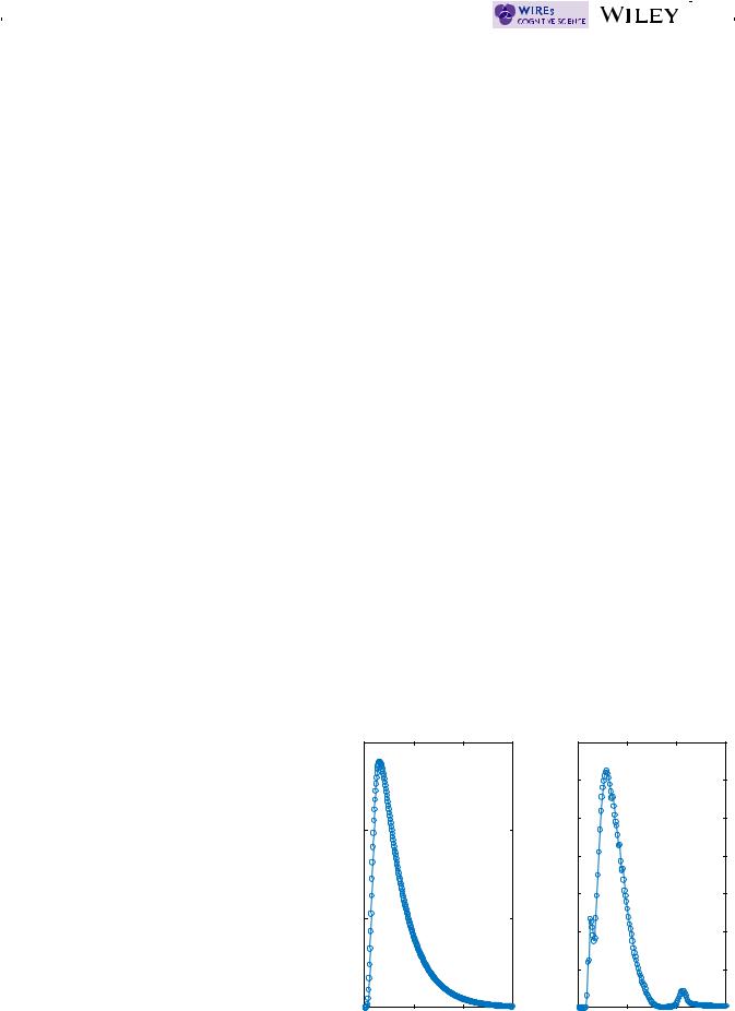
been observed by other researchers (Fuss & Navarro, 2013), and may constitute an adaptive reason for why a decision maker would implement a quantum rather than Markov random walk for decision making. Second, the quantum model has a small second mode, which is produced by oscillation and interference properties of the quantum dynamics. Empirically multimodal distributions have been interpreted as evidence for multiple stage processes (see, e.g., Pleskac & Wershbale, 2014); however, in this case there is only a single process. Furthermore, empirical distributions are often smoothed, which could make it difficult to detect a small second mode in the distribution.
The first comparison between models with regard to response times was carried out by Busemeyer et al. (2006). In that work, the distributions of response times were derived from quantum and Markov models by assuming that a choice was made as soon as the state was measured at a location beyond a specific criterion level. Measurements were assumed to occur every 10 ms to determine if the process had crossed the choice boundary by that time. This initial effort at comparing models in terms of response time predictions favored the Markov model, which was nearly equivalent to the well established diffusion decision model of response times (Ratcliff et al., 2016). Although this first comparison did not favor the quantum model, it did show that the quantum model was capable of providing reasonably accurate fits to the choice and response time distributions.
This early work comparing quantum and Markov models of response time was then followed up by subsequent developments by Fuss and Navarro (2013), who used a more general approach to modeling quantum dynamical systems. The previous work by Busemeyer et al. (2006) was limited by its use of what is called a “closed” quantum system that does not include any additional “noise” operators and always remains in a coherent (superposed) state. Fuss and Navarro (2013) implemented a quantum random walk that included quantum “noise” operators that generate partial decoherence, producing a decay into a part-quantum and part-classical system that mixed both von Neumann uncertainty (measurement uncertainty about where a superposition state will collapse) and classical uncertainty (uncertainty about which of several states a person is located). This type of “open” quantum system represents a potentially more realistic view of quantum random walk models (Yearsley, 2017), where the superposition state partially decoheres as a result of interactions with “noise” (as opposed to the “pure” coherent states presented above that are part of a closed quantum system without any “noise”). This partially coherent quantum model can be interpreted as a massively parallel cognitive architecture that involves both inhibitory and excitatory interactions between units (e.g., neurons or neural populations), as we might expect from neural representations of evidence. It turns out that this more general quantum walk model out-performed a simple diffusion model in fitting the response time distributions in a perceptual decisionmaking experiment (Gökaydin, Ma-Wyatt, Navarro, & Perfors, 2011).
With results running in both directions between Markov and quantum models, it is too early to say which type of model is more promising for modeling response times. Quantitative tests based on model fits may not produce a clear answer for distinguishing these two type of response time models. Instead, the quality of out-of-sample predictions like the generalization test (similar to that presented in the interference with double confidence ratings section) may be necessary to arbitrate between them. Nevertheless, the open quantum systems approach, inspired by the cooperative and competitive interactions between units representing evidence (neurons), appears a promising direction for developing better models of response times.
10 | PREFERENCE AND DISSONANCE
As mentioned at the beginning, Markov and quantum process are also applicable to understanding how preferences accumulate and evolve over time. A great deal of work has already been done applying Markov models to preference (Busemeyer, Gluth, Rieskamp, & Turner, 2019; Pleskac, Diederich, & Wallsten, 2015), but we are only beginning to apply quantum processes to preference evolution. Two initial applications are described below.
The quantum model is equally applicable whether the underlying scale is degrees of preference or degrees of belief, and so it makes extremely similar predictions regarding the effect of a binary choice on subsequent preference ratings as it does with confidence ratings. Namely, it suggests that preference ratings that follow a choice, when there is information processing between the choice and preference rating, should diverge from those that are not preceded by a choice as in the interference from choice on confidence study above. The effect of a decision on subsequent preferences that arises from the quantum walk models bears some interesting commonalities with other well-studied phenomena. In particular, the observation that making a decision results in different distributions of confidence judgments is reminiscent of work on cognitive dissonance that was applied to preference judgments (Festinger, 1957, 1964). In this work, a decision maker is offered a choice between two alternatives, and then is subsequently (after some delay following
suai.ru/our-contacts |
quantum |
machine |
|
learning |
||||
|
||||||||
|
BUSEMEYER ET AL. |
|
|
|
|
|
13 of 19 |
|
choice) asked to rate their preference between the choice options. The typical finding is that postchoice preference ratings favor the chosen alternative, relative to either prechoice preferences (Brehm, 1956) or to a preference elicited in absence of prior choice (Festinger & Walster, 1964).
The typical explanation for dissonance effects is one of motivated reasoning: A person is driven by conflict between internal states of preference (A and B are similar in value) and stated preference elicited via choice (A chosen over B) to change their degree of preference to favor the chosen option. However, this “bolstering” effect is sometimes preceded by an opposing “suppression” effect, where a chosen alternative is more weakly preferred to an alternative compared to cases where there is no decision between the options (Brehm & Wicklund, 1970; Festinger & Walster, 1964; Walster, 1964). Both of these effects are clearly at odds with a Markov account of preference representation, which suggests that making a decision by itself should not change alter an underlying preference state between a pair of options.
Conversely, the quantum dynamical models provide a natural explanation for these bolstering and suppression effects. Although the quantum account is not incompatible with the dissonance account of bolstering based on motivational processes, the quantum framework offers an alternative explanation for these effects. For example, White et al. (2014, 2016) used measurement effects with a (nondynamic) quantum model to account for decision biases that unfolded in sequential affective judgments.
Here, we take this work a step further by using a dynamical model to account for preferences measured at experimentally at different controlled points in time. According to quantum dynamics, the measurement of a choice at an early time point creates a cognitive state that interacts with subsequent accumulation dynamics. Therefore a quantum process predicts that a choice at an early time point naturally results in subsequent preferences that diverge from those produced by a no-choice condition. As with the choice-confidence interference study, we expect a paradigm eliciting choice and then preference to yield an interference effect where preference ratings in a no-choice condition systematically differed from those in a choice condition.
11 | OSCILLATION
One implication of the quantum approach to preference formation and dissonance is that it predicts bolstering and suppression effects should depend on the time at which preference ratings are elicited. The choice-confidence interference study used a relatively short timescale between choice and confidence ratings (maximum 1.5 s after choice), and generated an effect closer to suppression, where ratings were more extreme in the no-choice than in the choice condition. However, due to the oscillatory nature of quantum models, we also expect to find the reverse phenomenon of bolstering (choice > no-choice) when confidence or preference strength is elicited at a later point in time.
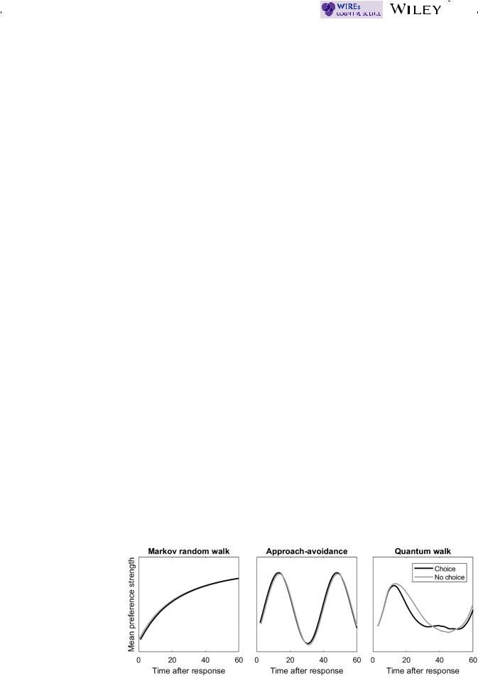
An example of model predictions for how preference should evolve over time for a Markov, a deterministic oscillator, and a quantum model are shown in Figure 7. As shown, the quantum model predicts that preference strength should oscillate over time, owing to the wave-like dynamics described in Table 1. Choice dampens the magnitude of these oscillations, leading to instances of both suppression (no-choice > choice, around 5–35 s after choice in Figure 7) and bolstering (choice > no-choice, around 25–50 s after choice in Figure 7). Naturally, the time at which each type of effect appears will depend on the stimuli used as choice alternatives, the individual characteristics of the decisionmaker, and thus the corresponding parameters of the model (such as drift rate and diffusion). Work exploring this unique oscillation prediction from the quantum model is still underway, but early suggestions are that oscillations do
F I G U R E 7 Expected time course of mean preference ratings generated from a typical Markov random walk model (left), a deterministic oscillating approach-avoidance model (middle), and quantum walk model (right)
