the belief-action state is implemented by the weight parameters {, µ} on the Win and Lose states, for first and second period respectively.

Finally the carry-over effect from first to second period on the U condition belief-action state is implemented by the weight parameter {}.

The Markov model therefore relies on 9 parameters to cover the process dynamics and the initial beliefs in both flow orders, both periods and all payoffs, amounting to providing theoretical values to 30 data points. In the Supplementary Materials section (SM 1) the full temporal evolution description of the belief-action state is provided for the full sample of participants who passed the attention test.

4.3. The quantum-like model

The quantum-like model applies a state vector to represent the belief-action state of the participant but instead of having probability components like in the Markov approach, it has probability amplitude components. These components can be complex valued and only lead to probabilities after taking the squared norm. In Appendix A, an elementary introduction to the application of the quantum formalism in cognition is given, which also provides an exposition of its close resemblance to the Markov formalism.

The similarity with the Markov model allows a fairly straightforward formulation of the quantum-like model that runs parallel to the previous section on the Markov model and only requires some clarification for a few distinct features.

The minimal representation of the gamble paradigm crosses the conditions for Win or Lose and the decision to Gamble or Stop. The associated belief-action state will be denoted as

where the amplitude components represent the respective belief support for first-stage gamble outcome condition combined with action-potential for different gamble decisions in the second-stage gamble. In the quantum-like model the probability for the participant to take the second-stage gamble is obtained by adding the modulus squared of the components for ‘Gamble in the secondstage and Won-first-stage belief’ and ‘Gamble in the second-stage and Lost-first-stage belief’

In general, since the belief-action states covers the full event space for the decisions Gamble and Stop and categories Win and Lose, the corresponding probabilities add up to unity:

which is the normalization of the belief-action state vector. In the quantum-like model the belief-action state at the moment of decision is realized through a measurement operation. In particular the outcome state for the decision to gamble is obtained through

the corresponding projector MGamble for the question ‘Take the second-stage gamble?’ and the projector MStop for ‘Stop the secondstage gamble?’.12

Notice that formally this projection matrix is identical to the selection matrix in the Markov model, Eq. (28). The modulus square of the projected vector for the measurement ‘Take the second-stage gamble?’ then gives the gamble probability, Eq. (35).

In the quantum-like model the process of change of the belief-action state occurs at the level of the probability amplitudes. The transforming effect of incoming information is controlled by the Hamiltonian operator H. Now the specific parameter positions in this matrix will cause the transfer of probability amplitude between the different vector components of the belief-action state. In the quantum-like case - due to the original relation of the Hamiltonian operator to the real-valued ‘energy’ of a system - the operator for change has to be Hermitian. This means the component Hij for transferring probability amplitude from vector component with index j to i has to be complex conjugated with respect to the component Hji, which transfers probability amplitude from component i to j. The Hermiticity requirement is expressed as H = H†. In the two stage gamble paradigm the main factor of transfer in the belief-action state depends on the condition of the outcome of the initial gamble. This information will re-distribute the Gamble or Stop components in the Win subspace and also the Gamble or Stop component in the Lose subspace. The transformation within the subspace of Win and subspace of Lose requires the two respective Hamiltonian sub matrices –satisfying the Hermitian condition;13

12Note that a projector is any matrix M which is idempotent, M2 = M. The projection occurs on the span of its eigenvectors. See also (Appendix A) for an elementary introduction to quantum modeling.

13A two-dimensional quantum-like model with Hamiltonian matrix, Eq. (39), allows to analytically calculate the unitary propagator U (t), Eq. (44), Broekaert et al., 2016),

17

J.B. Broekaert, et al. Cognitive Psychology 117 (2020) 101262

where . The encompassing Hamiltonian, with HW in the upper left matrix quadrant and with HL in the lower right quadrant, acts separately on the subspaces for Win and Lose

This type of Hamiltonian would keep Win-related and Lose-related belief amplitudes fully independent.

Similarly as in the Markov model the magnitude of the transfer process will depend on the utility of the second-stage gamble. In contrast to the driving parameters in the transition rate matrix of the Markov process, Eq. (23), in the Hamiltonian the driving parameters can be positive or negative valued. More generally we could also parametrise the Hamiltonian with complex valued parameters while assuring Hermiticity. To accommodate both signs, the parameters are modeled by a hyperbolic tangent (version of the logistic) function of the linear utility expression:

with X [.5, 1…4] and with scaling parameter s.

The assumed cognitive process –similar as to the Markov model– will mix the W and L beliefs under all first-stage gamble outcome conditions. In the Unknown first-stage outcome condition the uncertainty about loss or win engenders an uncertainty about Gambling or Stopping, but also in the Known first-stage outcome gambles mixing of Win and Lose beliefs will occur due to a contextual effect in the block. The mixing operator will cause attention switching between Win and Lose beliefs to happen concurrently with switching decisions for Gambling or Stopping. In practice the mixing Hamiltonian thus transfers action-potential from ‘Gamble on Win’ ( GW ) to ‘Stop on Lose’ ( SL) and, from ‘Stop on Win’ ( SW ) to ‘Gamble on Lose’ ( GL). The mixing dynamics corresponds to an explorative attention switching between potential outcomes of the gamble in which a switch between Win and Lose belief always correlates with a switch in the decision between to Gamble and to Stop in the second-stage gamble. These two correlated attention switching processes are implemented by

The full Hamiltonian matrix H, which implements the cognitive process for Win, Lose and Unknown condition is then composed

The temporal change of the belief-action state is produced by the unitary evolution operator U, and is itself driven by Hamiltonian operator H. The unitary operator satisfies the Schrödinger equation (Busemeyer & Bruza, 2012), in accordance with the dynamics of quantum theory

In the quantum-like model, the belief-action state at time t and under condition C of the initial stage gamble outcome is given by

The probability for taking the second-stage gamble under condition C is then obtained from the evolved belief-action state at the time of measurement, by projecting with Mgamble for ‘taking the second-stage gamble’ and taking the modulus square of that outcome

The time of measurement is fixed to the conventional choice t = /2, corresponding to the choice of measurement time in the Markov model, Eq. (29). Since the time-scale of the evolution, Eq. (45), for the cognitive realm is undefined and since no response time observations are involved, a designated time of measurement can be fixed by convention. Notice too that both in the Markov model

(footnote continued)

In contrast to the Markov propagator, the oscillatory evolution of the quantum-like propagator requires a choice of measurement time that remains within the system’s period.

18

and in the quantum-like model the optimized parameter fitting will be adapted to this conventional time choice.

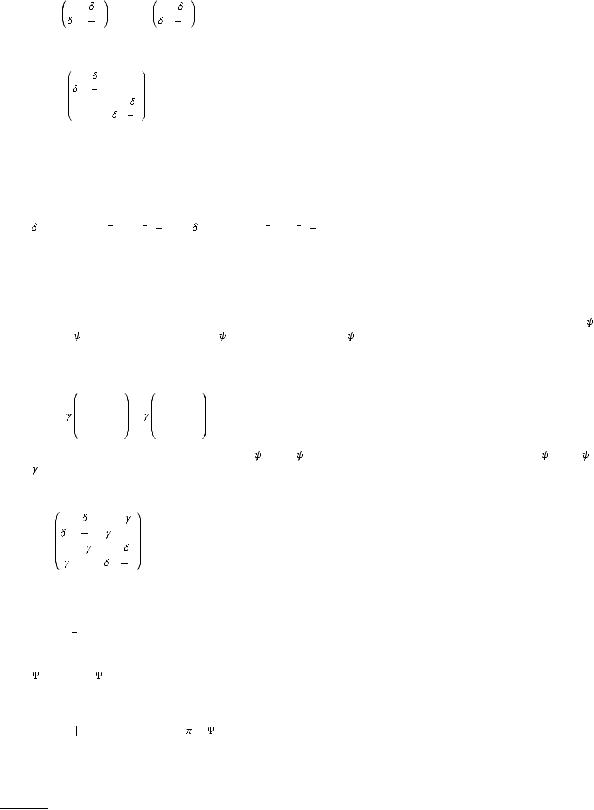
For each of the two periods for decision making in each flow order (K-to-U and U-to-K) a separate final belief-action state will be obtained. These final states will differ due to their respective initial belief-action states. Since the quantum-like model uses vectors of probability amplitudes - that require modulus squaring for probabilities - it is more transparent to write the 4-dimensional vectors as a tensor product of two 2-dimensional vectors, the first one for category Win/Lose and the second one for decision Gamble/Stop (see Supplementary Materials, Eq. (A2) for details).In the first period, the initial belief-action states on Win, respectively Lose, outcome condition of the first-stage gamble are formally given by the vectors;14

where is a weight parameter, 0 1. Should = 1 then these respective states are precisely allocated to the Win and Lose components, while the probability to Gamble or Stop for each of them is uniformly .5, as can easily be verified by squaring the entries in the Gamble/Stop vector. In the block with Known outcome conditions the participant is exposed to both Win and Lose outcome gambles. These two conditions create a mutual context for each gamble. The context effect will be present when < 1 and expresses the idea that the information on the condition of the first-stage gamble is only partially integrated into the belief-action state.

The initial belief-action state –in first period– in the Unknown outcome case of the first-stage gamble is expressed as

11

which reveals that the belief support for Win or Lose is uniform and also the action-potential for the Gamble or Stop decision is indifferent due to lack of any prior experience with gambles. The state is caused by the uncertainty due to missing information on the first-stage outcome in the Unknown-outcome condition.

In the second period the context effect is modified by the carry-over effect, hence the initial state now depends on the block’s gamble condition as well as on the participant’s history of the first period. The initial belief-action states for Win and Lose conditions will reflect residual belief support for the opposite condition modified by the carry-over from the previous period

Since the initial belief-action state in the second period is influenced by the first block’s condition, in the Unknown condition the belief-action state will be a superposition of the two states for the possible outcome conditions W and L of the Known outcome conditioned gambles block. In particular, the quantum-formalism allows to weight both conditions equally but also to include a relative complex phase between the two states for Win and Lose. The sign and amplitude of this phase allows for constructive or destructive interference between the two states and thus brings about a subjective tendency towards either of the known outcome beliefs

interference of belief-action states indicates a susceptibility for an amplifying or reducing relation between beliefs. In the event of ‘decoherence’ between these belief-action states –by their reduction to separate contexts– interference between them will be diminished or impeded. In the second period the probability for taking the second-stage gamble under either of conditions {W , L, U} is

again obtained according to Eq. (46), by projecting the evolved belief-action state using Mgamble, the projector for ‘taking the secondstage gamble’, and taking the modulus squared.

In the Supplementary Materials, (SM 2), a graph of the time development of the probability of the decision process for the secondstage gamble shows the build up of the gamble probabilities emerging from each of the initial belief-action states.

Parametrization. The quantum-like model requires a parametrization that closely resembles the parametrization of the Markov model. It requires the four dynamical parameters for the driving utility difference of the second-stage gamble for the two conditions of Win and Lose, namely {0W , 1W } and {0L, 1L}. Also the effect of the utility difference on the decision is controlled by a sensitivity

14 The tensor product notation is used here to distinguish more easily the effect of the parameter on the belief support in the Win/Lose evaluation. The two dimensional vector for Win/Lose appears as the left factor of the tensor product, the right factor is the two dimensional vector for Gamble/ Stop. Both subspace vectors can be blended into the four dimensional vector according to the usual rule

ac

adbc = (ab) (dc ). bd

19