

- •CONTENTS
- •Preface
- •To the Student
- •Diagnostic Tests
- •1.1 Four Ways to Represent a Function
- •1.2 Mathematical Models: A Catalog of Essential Functions
- •1.3 New Functions from Old Functions
- •1.4 Graphing Calculators and Computers
- •1.6 Inverse Functions and Logarithms
- •Review
- •2.1 The Tangent and Velocity Problems
- •2.2 The Limit of a Function
- •2.3 Calculating Limits Using the Limit Laws
- •2.4 The Precise Definition of a Limit
- •2.5 Continuity
- •2.6 Limits at Infinity; Horizontal Asymptotes
- •2.7 Derivatives and Rates of Change
- •Review
- •3.2 The Product and Quotient Rules
- •3.3 Derivatives of Trigonometric Functions
- •3.4 The Chain Rule
- •3.5 Implicit Differentiation
- •3.6 Derivatives of Logarithmic Functions
- •3.7 Rates of Change in the Natural and Social Sciences
- •3.8 Exponential Growth and Decay
- •3.9 Related Rates
- •3.10 Linear Approximations and Differentials
- •3.11 Hyperbolic Functions
- •Review
- •4.1 Maximum and Minimum Values
- •4.2 The Mean Value Theorem
- •4.3 How Derivatives Affect the Shape of a Graph
- •4.5 Summary of Curve Sketching
- •4.7 Optimization Problems
- •Review
- •5 INTEGRALS
- •5.1 Areas and Distances
- •5.2 The Definite Integral
- •5.3 The Fundamental Theorem of Calculus
- •5.4 Indefinite Integrals and the Net Change Theorem
- •5.5 The Substitution Rule
- •6.1 Areas between Curves
- •6.2 Volumes
- •6.3 Volumes by Cylindrical Shells
- •6.4 Work
- •6.5 Average Value of a Function
- •Review
- •7.1 Integration by Parts
- •7.2 Trigonometric Integrals
- •7.3 Trigonometric Substitution
- •7.4 Integration of Rational Functions by Partial Fractions
- •7.5 Strategy for Integration
- •7.6 Integration Using Tables and Computer Algebra Systems
- •7.7 Approximate Integration
- •7.8 Improper Integrals
- •Review
- •8.1 Arc Length
- •8.2 Area of a Surface of Revolution
- •8.3 Applications to Physics and Engineering
- •8.4 Applications to Economics and Biology
- •8.5 Probability
- •Review
- •9.1 Modeling with Differential Equations
- •9.2 Direction Fields and Euler’s Method
- •9.3 Separable Equations
- •9.4 Models for Population Growth
- •9.5 Linear Equations
- •9.6 Predator-Prey Systems
- •Review
- •10.1 Curves Defined by Parametric Equations
- •10.2 Calculus with Parametric Curves
- •10.3 Polar Coordinates
- •10.4 Areas and Lengths in Polar Coordinates
- •10.5 Conic Sections
- •10.6 Conic Sections in Polar Coordinates
- •Review
- •11.1 Sequences
- •11.2 Series
- •11.3 The Integral Test and Estimates of Sums
- •11.4 The Comparison Tests
- •11.5 Alternating Series
- •11.6 Absolute Convergence and the Ratio and Root Tests
- •11.7 Strategy for Testing Series
- •11.8 Power Series
- •11.9 Representations of Functions as Power Series
- •11.10 Taylor and Maclaurin Series
- •11.11 Applications of Taylor Polynomials
- •Review
- •APPENDIXES
- •A Numbers, Inequalities, and Absolute Values
- •B Coordinate Geometry and Lines
- •E Sigma Notation
- •F Proofs of Theorems
- •G The Logarithm Defined as an Integral
- •INDEX

A10 |
|||| APPENDIX B |
COORDINATE GEOMETRY AND LINES |
57–58 Solve for x, assuming a, b, and c are positive constants. |
||
57. |
a bx c bc |
58. a bx c 2a |
|
|
|
59–60 Solve for x, assuming a, b, and c are negative constants.
60. ax b b c
61.Suppose that x 2 0.01 and y 3 0.04. Use the Triangle Inequality to show that x y 5 0.05.
62. |
Show that if x 3 21 , then 4x 13 3. |
||
63. |
Show that if a b, then a |
a b |
b. |
|
|||
2 |
|||
64. |
Use Rule 3 to prove Rule 5 of (2). |
|
|
65. |
Prove that ab a b . [Hint: Use Equation 4.] |
||||
|
|
a |
a |
||
66. |
Prove that |
|
|
|
. |
b |
b |
||||
67. |
Show that if 0 a b, then a 2 b 2. |
||||
68. |
Prove that x y x y . [Hint: Use the Triangle |
||||
|
Inequality with a x y and b y.] |
||||
69.Show that the sum, difference, and product of rational numbers are rational numbers.
70.(a) Is the sum of two irrational numbers always an irrational number?
(b)Is the product of two irrational numbers always an irrational number?
B COORDINATE GEOMETRY AND LINES
Just as the points on a line can be identified with real numbers by assigning them coordinates, as described in Appendix A, so the points in a plane can be identified with ordered pairs of real numbers. We start by drawing two perpendicular coordinate lines that intersect at the origin O on each line. Usually one line is horizontal with positive direction to the right and is called the x-axis; the other line is vertical with positive direction upward and is called the y-axis.
Any point P in the plane can be located by a unique ordered pair of numbers as follows. Draw lines through P perpendicular to the x- and y-axes. These lines intersect the axes in points with coordinates a and b as shown in Figure 1. Then the point P is assigned the ordered pair a, b . The first number a is called the x-coordinate of P; the second number b is called the y-coordinate of P. We say that P is the point with coordinates a, b , and we denote the point by the symbol P a, b . Several points are labeled with their coordinates in Figure 2.
|
|
|
|
y |
|
|
|
|
|
P(a,b) |
|
|
|
y |
|
|
|
|
|
|
|
|
|||||||
|
|
|
|
|
|
|
|
|
|
|
|
|
|
|
|
|
|
|
|||||||||||
|
|
b |
4 |
|
|
|
|
|
|
|
4 |
|
|
(1,3) |
|
|
|
|
|||||||||||
|
|
3 |
|
|
|
|
|
|
|
|
|
|
|
|
3 |
|
|
|
|
|
|
||||||||
|
|
|
|
|
|
|
|
|
|
|
|
|
|
|
|
|
|
|
|
|
|||||||||
|
II |
2 |
|
|
|
|
I |
|
|
|
|
|
(_2,2) |
|
|
|
|
|
|
|
|
|
|
||||||
|
|
|
|
|
|
|
|
|
|
2 |
|
|
|
|
|
|
|
|
|
||||||||||
|
|
|
|
|
|
|
|
|
|
|
|
|
|
|
|
|
|
|
|
|
|
|
|
||||||
|
|
|
1 |
|
|
|
|
|
|
|
|
|
|
|
|
1 |
|
|
|
|
|
|
|
|
|
||||
|
|
|
|
|
|
|
|
|
|
|
|
|
|
|
(5,0) |
|
|||||||||||||
|
|
|
|
|
|
|
|
|
|
|
|
|
|
|
|
|
|
|
|
|
|
|
|||||||
|
|
|
|
|
|
|
|
|
|
|
|
|
|
|
|
|
|
|
|
|
|
|
|
|
|
|
|
|
|
|
|
|
|
|
|
|
|
|
|
|
|
|
|
|
|
|
|
|
|
|
|
|
|
|
|
|
|
||
_3 _2 _ |
1 O |
1 2 3 |
4 5 x |
_3 _2 _ |
1 0 |
|
|
1 2 3 4 5 x |
|||||||||||||||||||||
|
|
|
_1 |
|
|
|
|
|
|
|
|
|
|
|
|
_1 |
|
|
|
|
|
|
|
|
|
||||
|
|
|
|
|
|
|
|
a |
|
|
|
|
|
|
|
|
|
||||||||||||
|
|
|
_2 |
|
|
|
|
|
|
_2 |
|
|
|
|
|
|
|
|
|
||||||||||
|
III |
_3 |
|
|
|
|
IV |
(_3,_2) |
|
|
|
|
|
|
|
|
|
|
|||||||||||
|
|
|
|
|
|
|
|
|
|
|
|
|
|
|
_3 |
|
|
(2,_4) |
|
|
|
||||||||
|
|
|
|
|
|
|
|
|
|
|
|
|
|
|
|
|
|
|
|
||||||||||
|
|
|
_4 |
|
|
|
|
|
|
|
|
|
|
|
|
_4 |
|
|
|
|
|
||||||||
|
|
|
|
|
|
|
|
|
|
|
|
|
|
|
|
|
|
|
|
||||||||||
|
|
|
|
|
|
|
|
|
|
|
|
|
|
|
|
|
|
|
|
|
|
|
|
|
|
|
|
|
|
FIGURE 1 |
|
|
|
|
|
|
|
|
|
|
FIGURE 2 |
|
|
|
|
|
|
|
|
||||||||||
By reversing the preceding process we can start with an ordered pair a, b and arrive at the corresponding point P. Often we identify the point P with the ordered pair a, b and refer to “the point a, b .” [Although the notation used for an open interval a, b is the

APPENDIX B COORDINATE GEOMETRY AND LINES |||| A11
same as the notation used for a point a, b , you will be able to tell from the context which meaning is intended.]
This coordinate system is called the rectangular coordinate system or the Cartesian coordinate system in honor of the French mathematician René Descartes (1596–1650), even though another Frenchman, Pierre Fermat (1601–1665), invented the principles of analytic geometry at about the same time as Descartes. The plane supplied with this coordinate system is called the coordinate plane or the Cartesian plane and is denoted by 2.
The x- and y-axes are called the coordinate axes and divide the Cartesian plane into four quadrants, which are labeled I, II, III, and IV in Figure 1. Notice that the first quadrant consists of those points whose x- and y-coordinates are both positive.
EXAMPLE 1 Describe and sketch the regions given by the following sets. |
||
(a) x, y x 0 |
(b) x, y y 1 |
(c ) { x, y y 1} |
SOLUTION
(a) The points whose x-coordinates are 0 or positive lie on the y-axis or to the right of it as indicated by the shaded region in Figure 3(a).
|
|
|
|
|
y |
|
|
|
|
|
|
|
|
|
|
y |
|
|
y=1 |
|
|
|
|
|
|
|
y |
|
y=1 |
|
|
||||||
|
|
|
|
|
|
|
|
|
|
|
|
|
|
||||||||||||||||||||||||
|
|
|
|
|
|
|
|
|
|
|
|
|
|
|
|
|
|
|
|
|
|
|
|
|
|
|
|
|
|
|
|
||||||
|
|
|
|
|
|
|
|
|
|
|
|
|
|
|
|
|
|
|
|
|
|
|
|
|
|
|
|
|
|
|
|
||||||
|
|
|
|
|
|
|
|
|
|
|
|
|
|
|
|
|
|
|
|
|
|
|
|
|
|
|
|
|
|
|
|
|
|
|
|
|
|
|
|
|
|
|
|
|
|
|
|
|
|
|
|
|
|
|
|
|
|
|
|
|
|
|
|
|
|
|
|
|
|
|
|
|
|
||
|
|
|
|
|
|
|
|
|
|
|
|
|
|
|
|
|
|
|
|
|
|
|
|
|
|
|
|
|
|
|
|
|
|
|
|
|
|
|
|
|
|
|
0 |
|
|
|
|
|
x |
|
|
|
|
0 |
|
|
|
|
|
|
|
x |
|
|
|
|
0 |
|
|
|
|
|
x |
||
|
|
|
|
|
|
|
|
|
|
|
|
|
|
|
|
|
|
|
|
|
|
|
|
|
|
|
|
|
|
|
|
|
|
|
|
|
|
|
|
|
|
|
|
|
|
|
|
|
|
|
|
|
|
|
|
|
|
|
|
|
|
|
|
|
|
|
|
|
|
|
y=_1 |
|
|
||
|
|
|
|
|
|
|
|
|
|
|
|
|
|
|
|
|
|
|
|
|
|
|
|
|
|
|
|
|
|
|
|
|
|
|
|
|
|
|
|
|
|
|
|
|
|
|
|
|
|
|
|
|
|
|
|
|
|
|
|
|
|
|
|
|
|
|
|
|
|
|
|
|
|
|
|
FIGURE 3 |
|
|
|
|
(a) x 0 |
|
|
|
|
|
|
|
(b) y=1 |
|
|
|
|
|
|
|
(c) |y|<1 |
|
|
||||||||||||||
y
P™(¤,fi)
fi
|fi-›|
P¡(⁄,›)
› 


 |¤-⁄|
|¤-⁄| 
 P£(¤,›)
0 |
⁄ |
¤ |
x |
FIGURE 4
(b)The set of all points with y-coordinate 1 is a horizontal line one unit above the x-axis [see Figure 3(b)].
(c)Recall from Appendix A that
y 1 if and only if 1 y 1
The given region consists of those points in the plane whose y-coordinates lie between1 and 1. Thus the region consists of all points that lie between (but not on) the horizontal lines y 1 and y 1. [These lines are shown as dashed lines in Figure 3(c) to indicate that the points on these lines don’t lie in the set.] M
Recall from Appendix A that the distance between points a and b on a number line isa b b a . Thus the distance between points P1 x1, y1 and P3 x2, y1 on a horizontal line must be x2 x1 and the distance between P2 x2, y2 and P3 x2, y1 on a vertical line must be y2 y1 . (See Figure 4.)
To find the distance P1P2 between any two points P1 x1, y1 and P2 x2, y2 , we note that triangle P1P2 P3 in Figure 4 is a right triangle, and so by the Pythagorean Theorem we have
P1P2 s P1P3 2 P2P3 2 s x2 x1 2 y2 y1 2
s x2 x1 2 y2 y1 2

A12 |||| APPENDIX B COORDINATE GEOMETRY AND LINES
y |
|
|
|
L |
|
|
|
||||
|
|
|
P™(x™,y™) |
||
|
|
|
|
Îy=fi-› |
|
|
|
|
|
||
P¡(x¡,y¡) |
|
=rise |
|||
|
|
|
Îx=¤-⁄ |
||
|
|
|
|||
|
|
|
=run |
||
|
|
|
|
|
|
0 |
|
|
|
x |
|
|
|
|
|
|
|
FIGURE 5
y |
m=5 |
|
|
|
m=2 |
|
|
|
m=1 |
|
|
|
m= |
1 |
|
|
|
2 |
|
|
m=0 |
|
|
|
m=_ |
1 |
|
|
|
|
2 |
0 |
m=_1 |
|
x |
|
m=_2 |
|
|
|
m=_5 |
|
|
FIGURE 6
1DISTANCE FORMULA The distance between the points P1 x1, y1 and P2 x2, y2 is
P1P2 s x2 x1 2 y2 y1 2
EXAMPLE 2 The distance between 1, 2 and 5, 3 is |
|
s 5 1 2 3 2 2 s42 52 s41 |
M |
LINES
We want to find an equation of a given line L; such an equation is satisfied by the coordinates of the points on L and by no other point. To find the equation of L we use its slope, which is a measure of the steepness of the line.
2 DEFINITION The slope of a nonvertical line that passes through the points |
|||||
P1 x1, y1 and P2 x2, y2 is |
|
|
|
|
|
m |
y |
|
y2 |
y1 |
|
x |
x2 |
x1 |
|||
The slope of a vertical line is not defined.
Thus the slope of a line is the ratio of the change in y, y, to the change in x, x. (See Figure 5.) The slope is therefore the rate of change of y with respect to x. The fact that the line is straight means that the rate of change is constant.
Figure 6 shows several lines labeled with their slopes. Notice that lines with positive slope slant upward to the right, whereas lines with negative slope slant downward to the right. Notice also that the steepest lines are the ones for which the absolute value of the slope is largest, and a horizontal line has slope 0.
Now let’s find an equation of the line that passes through a given point P1 x1, y1 and has slope m. A point P x, y with x x1 lies on this line if and only if the slope of the line through P1 and P is equal to m; that is,
y y1 m x x1
This equation can be rewritten in the form
y y1 m x x1
and we observe that this equation is also satisfied when x x1 and y y1. Therefore it is an equation of the given line.
3 POINT-SLOPE FORM OF THE EQUATION OF A LINE An equation of the line passing through the point P1 x1, y1 and having slope m is
y y1 m x x1
|
|
|
|
|
|
|
|
|
|
|
|
APPENDIX B COORDINATE GEOMETRY AND LINES |||| |
A13 |
||||||
|
|
|
|
|
|
|
|
|
|
EXAMPLE 3 Find an equation of the line through 1, 7 with slope 21 . |
|
||||||||
|
|
|
|
|
|
|
|
|
|
SOLUTION |
Using 3 with m 21 , x1 1, and y1 7, we obtain an equation of the line |
||||||||
|
|
|
|
|
|
|
|
|
|
as |
|
|
|
|
|
|
|
|
|
|
|
|
|
|
|
|
|
|
|
|
|
y 7 21 x 1 |
|
||||||
|
|
|
|
|
|
|
|
|
|
which we can rewrite as |
|
|
|
|
|
|
|
||
|
|
|
|
|
|
|
|
|
|
|
2y 14 x 1 |
or |
x 2y 13 0 |
M |
|||||
|
|
|
|
|
|
|
|
|
|
EXAMPLE 4 Find an equation of the line through the points 1, 2 and 3, 4 . |
|
||||||||
|
|
|
|
|
|
|
|
|
|
SOLUTION |
By Definition 2 the slope of the line is |
|
|
|
|
|
|||
|
|
|
|
|
|
|
|
|
|
|
|
m |
4 2 |
3 |
|
|
|
||
|
|
|
|
|
|
|
|
|
|
|
|
|
|
|
|
|
|
||
|
|
|
|
|
|
|
|
|
|
|
3 1 |
2 |
|
||||||
|
|
|
|
|
|
|
|
|
|
Using the point-slope form with x1 1 and y1 2, we obtain |
|
||||||||
|
|
|
|
|
|
|
|
|
|
|
|
y 2 23 x 1 |
|
||||||
|
|
|
|
|
|
|
|
|
|
which simplifies to |
3x 2y 1 |
M |
|||||||
|
y |
|
|
|
|
|
|
Suppose a nonvertical line has slope m and y-intercept b. (See Figure 7.) This means it |
|||||||||||
|
|
|
|
|
|
|
|
|
|
intersects the y-axis at the point 0, b , so the point-slope form of the equation of the line, |
|||||||||
|
b |
|
y=mx+b |
|
|
|
with x1 0 and y1 b, becomes |
|
|
|
|
|
|
|
|||||
|
|
|
|
|
|
|
|
|
|
y b m x 0 |
|
||||||||
|
|
|
|
|
|
|
|
|
|
|
|
|
|||||||
|
|
|
|
|
|
|
|
|
|
This simplifies as follows. |
|
|
|
|
|
|
|
||
0 |
|
|
|
|
|
|
x |
|
|
|
|
|
|
|
|||||
|
|
|
|
|
|
|
|
|
|
|
|
|
|
|
|
||||
|
FIGURE 7 |
|
|
|
|
|
|
|
|
|
|
|
|
|
|
|
|||
|
|
|
|
|
|
4 |
SLOPE-INTERCEPT FORM OF THE EQUATION OF A LINE An equation of the line |
|
|||||||||||
|
|
|
|
|
|
|
|
|
|
with slope m and y-intercept b is |
|
|
|
|
|
|
|
||
|
|
|
|
|
|
|
|
|
|
|
|
|
y mx b |
|
|||||
|
y |
|
|
|
|
|
|
|
|
|
|
|
|||||||
|
|
|
|
|
|
|
|
In particular, if a line is horizontal, its slope is m 0, so its equation is y b, where |
|||||||||||
|
|
|
|
|
|
|
|||||||||||||
|
|
|
|
|
|
y=b |
|
|
|
b is the y-intercept (see Figure 8). A vertical line does not have a slope, but we can write |
|||||||||
|
b |
|
|
|
|
|
|
|
its equation as x a, where a is the x-intercept, because the x-coordinate of every point |
||||||||||
|
|
|
|
|
|
x=a |
|
|
|
on the line is a. |
|
|
|
|
|
|
|
||
|
|
|
|
|
|
|
|
|
Observe that the equation of every line can be written in the form |
|
|||||||||
|
|
|
|
|
|
|
|
|
|
|
|||||||||
|
|
|
|
|
|
|
|
|
|
|
|
|
|
|
|
|
|
||
0 |
|
|
|
a |
|
x |
|
|
|
|
|
|
|
|
|
|
|||
5 |
|
Ax By C 0 |
|
|
|||||||||||||||
|
|
|
|
|
|
|
|
|
|
|
|
|
|||||||
FIGURE 8 |
|
|
|
|
|
|
|
|
|||||||||||
|
|
|
|
|
|
|
|
|
|
|
|
|
|
|
|||||
|
|
|
|
|
because a vertical line has the equation x a or x a 0 (A 1, B 0, C a) and |
||||||||||||||
|
|
|
|
|
|
|
|
|
|
||||||||||
|
|
|
|
|
|
|
|
|
|
a nonvertical line has the equation y mx b or mx y b 0 (A m, B 1, |
|||||||||
|
|
|
|
|
|
|
|
|
|
C b). Conversely, if we start with a general first-degree equation, that is, an equation |
|||||||||
|
|
|
|
|
|
|
|
|
|
of the form (5), where A, B, and C are constants and A and B are not both 0, then we can |
|||||||||
|
|
|
|
|
|
|
|
|
|
show that it is the equation of a line. If B 0, the equation becomes Ax C 0 or |
|||||||||
|
|
|
|
|
|
|
|
|
|
x C A, which represents a vertical line with x-intercept C A. If B 0, the equation |
|||||||||
A14 |||| APPENDIX B COORDINATE GEOMETRY AND LINES
y
0
 (0,_3)
FIGURE 9
y
2.5
y |
|
|
= |
|
|
_ |
1 |
|
2 |
x |
|
|
+ |
5 |
|
2 |
|
|
|
0
FIGURE 10
15 5y= 3x-
(5,0) x
5x
can be rewritten by solving for y:
y A x C B B
and we recognize this as being the slope-intercept form of the equation of a line (m A B, b C B). Therefore an equation of the form (5) is called a linear equation or the general equation of a line. For brevity, we often refer to “the line Ax By C 0” instead of “the line whose equation is Ax By C 0.”
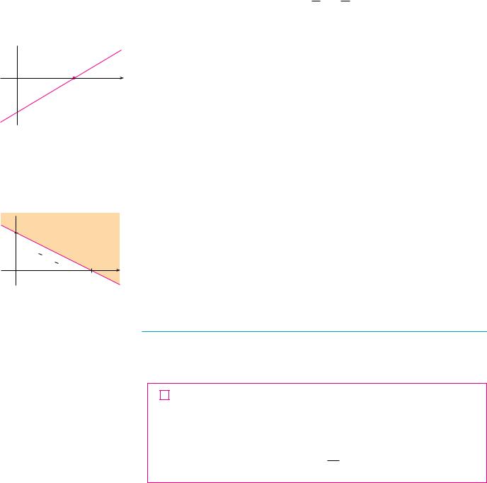
EXAMPLE 5 Sketch the graph of the equation 3x 5y 15.
SOLUTION Since the equation is linear, its graph is a line. To draw the graph, we can simply find two points on the line. It’s easiest to find the intercepts. Substituting y 0 (the equation of the x-axis) in the given equation, we get 3x 15, so x 5 is the x-intercept.
Substituting x 0 in the equation, we see that the y-intercept is 3. This allows us to |
|
sketch the graph as in Figure 9. |
M |
EXAMPLE 6 Graph the inequality x 2y 5.
SOLUTION We are asked to sketch the graph of the set x, y x 2y 5 and we do so by solving the inequality for y:
x 2y 5 |
|
2y x 5 |
|
y 21 x 25 |
|
Compare this inequality with the equation y 21 x 25 , which represents a line with |
|
slope 21 and y-intercept 25 . We see that the given graph consists of points whose |
|
y-coordinates are larger than those on the line y 21 x 25 . Thus the graph is the |
|
region that lies above the line, as illustrated in Figure 10. |
M |
PARALLEL AND PERPENDICULAR LINES
Slopes can be used to show that lines are parallel or perpendicular. The following facts are proved, for instance, in Precalculus: Mathematics for Calculus, Fifth Edition by Stewart, Redlin, and Watson (Thomson Brooks Cole, Belmont, CA, 2006).
6PARALLEL AND PERPENDICULAR LINES
1.Two nonvertical lines are parallel if and only if they have the same slope.
2.Two lines with slopes m1 and m2 are perpendicular if and only if m1m2 1; that is, their slopes are negative reciprocals:
m2
1
m1
EXAMPLE 7 Find an equation of the line through the point 5, 2 that is parallel to the line 4x 6y 5 0.
SOLUTION The given line can be written in the form
y 23 x 56

APPENDIX B COORDINATE GEOMETRY AND LINES |||| A15
which is in slope-intercept form with m 23 . Parallel lines have the same slope, so the required line has slope 23 and its equation in point-slope form is
y 2 23 x 5
We can write this equation as 2x 3y 16. M
EXAMPLE 8 Show that the lines 2x 3y 1 and 6x 4y 1 0 are perpendicular.
SOLUTION The equations can be written as
y 32 x 31 |
and |
y 23 x 41 |
from which we see that the slopes are |
|
|
m1 32 |
and |
m2 23 |
Since m1m2 1, the lines are perpendicular. |
M |
|
B EXERCISES
1–6 Find the distance between the points.
1. |
1, 1 , |
4, 5 |
2. |
1, 3 , 5, 7 |
3. |
6, 2 , 1, 3 |
4. |
1, 6 , 1, 3 |
|
5. |
2, 5 , |
4, 7 |
6. |
a, b , b, a |
|
|
|
|
|
7–10 Find the slope of the line through P and Q.
7. |
P 1, 5 , |
Q 4, 11 |
8. |
P 1, 6 , Q 4, 3 |
9. |
P 3, 3 , |
Q 1, 6 |
10. |
P 1, 4 , Q 6, 0 |
|
|
|
|
|
11.Show that the triangle with vertices A 0, 2 , B 3, 1 , and C 4, 3 is isosceles.
12.(a) Show that the triangle with vertices A 6, 7 , B 11, 3 , and C 2, 2 is a right triangle using the converse of the Pythagorean Theorem.
(b)Use slopes to show that ABC is a right triangle.
(c)Find the area of the triangle.
13.Show that the points 2, 9 , 4, 6 , 1, 0 , and 5, 3 are the vertices of a square.
14.(a) Show that the points A 1, 3 , B 3, 11 , and C 5, 15
are collinear (lie on the same line) by showing that
AB BC AC .
(b) Use slopes to show that A, B, and C are collinear.
15. Show that A 1, 1 , B 7, 4 , C 5, 10 , and D 1, 7 are vertices of a parallelogram.
16. Show that A 1, 1 , B 11, 3 , C 10, 8 , and D 0, 6 are vertices of a rectangle.
17–20 Sketch the graph of the equation.
17. x 3 18. y 2
19. xy 0 |
20. y 1 |
21–36 Find an equation of the line that satisfies the given
conditions. |
|
|
21. |
Through 2, 3 , |
slope 6 |
22. |
Through 1, 4 , |
slope 3 |
23. |
Through 1, 7 , |
slope 32 |
24. |
Through 3, 5 , slope 27 |
|
25.Through 2, 1 and 1, 6
26.Through 1, 2 and 4, 3
27.Slope 3, y-intercept 2
28.Slope 25, y-intercept 4
29. |
x-intercept 1, |
y-intercept 3 |
30. |
x-intercept 8, |
y-intercept 6 |
31.Through 4, 5 , parallel to the x-axis
32.Through 4, 5 , parallel to the y-axis
33.Through 1, 6 , parallel to the line x 2y 6
34.y-intercept 6, parallel to the line 2x 3y 4 0
35.Through 1, 2 , perpendicular to the line 2x 5y 8 0
36.Through (12 , 23 ), perpendicular to the line 4x 8y 1
37– 42 Find the slope and y-intercept of the line and draw its graph.
37. x 3y 0 |
38. 2x 5y 0 |
A16 |||| APPENDIX C GRAPHS OF SECOND-DEGREE EQUATIONS
39. |
y 2 |
40. |
2x 3y 6 0 |
41. |
3x 4y 12 |
42. |
4x 5y 10 |
|
|||
43–52 Sketch the region in the xy-plane. |
|||
43. |
x, y x 0 |
44. |
x, y y 0 |
45. |
x, y xy 0 |
46. |
x, y x 1 and y 3 |
47.{ x, y x 2}
48.{ x, y x 3 and y 2}
49.x, y 0 y 4 and x 2
50.x, y y 2x 1
51.x, y 1 x y 1 2x
52.{ x, y x y 12 x 3 }
53.Find a point on the y-axis that is equidistant from 5, 5
and 1, 1 .
54.Show that the midpoint of the line segment from P1 x1, y1 to
P2 x2, y2 is
x1 2 x2 , y1 2 y2
55. Find the midpoint of the line segment joining the given points.
(a) 1, 3 and 7, 15 (b) 1, 6 and 8, 12
56.Find the lengths of the medians of the triangle with vertices A 1, 0 , B 3, 6 , and C 8, 2 . (A median is a line segment from a vertex to the midpoint of the opposite side.)
57.Show that the lines 2x y 4 and 6x 2y 10 are not parallel and find their point of intersection.
58.Show that the lines 3x 5y 19 0 and 10x 6y 50 0 are perpendicular and find their point of intersection.
59.Find an equation of the perpendicular bisector of the line segment joining the points A 1, 4 and B 7, 2 .
60.(a) Find equations for the sides of the triangle with vertices
P 1, 0 , Q 3, 4 , and R 1, 6 .
(b)Find equations for the medians of this triangle. Where do they intersect?
61.(a) Show that if the x- and y-intercepts of a line are nonzero numbers a and b, then the equation of the line can be put in the form
x y 1 a b
This equation is called the two-intercept form of an equation of a line.
(b)Use part (a) to find an equation of the line whose x-intercept is 6 and whose y-intercept is 8.
62.A car leaves Detroit at 2:00 PM, traveling at a constant speed west along I-96. It passes Ann Arbor, 40 mi from Detroit, at 2:50 PM.
(a)Express the distance traveled in terms of the time elapsed.
(b)Draw the graph of the equation in part (a).
(c)What is the slope of this line? What does it represent?
CGRAPHS OF SECOND-DEGREE EQUATIONS
In Appendix B we saw that a first-degree, or linear, equation Ax By C 0 represents a line. In this section we discuss second-degree equations such as
x2 y2 1 |
y x2 |
1 |
x2 |
|
y |
2 |
1 |
x2 y2 1 |
|
4 |
|
||||||
|
|
9 |
|
|
|
|
||
which represent a circle, a parabola, an ellipse, and a hyperbola, respectively.
The graph of such an equation in x and y is the set of all points x, y that satisfy the equation; it gives a visual representation of the equation. Conversely, given a curve in the xy-plane, we may have to find an equation that represents it, that is, an equation satisfied by the coordinates of the points on the curve and by no other point. This is the other half of the basic principle of analytic geometry as formulated by Descartes and Fermat. The idea is that if a geometric curve can be represented by an algebraic equation, then the rules of algebra can be used to analyze the geometric problem.
CIRCLES
As an example of this type of problem, let’s find an equation of the circle with radius r and center h, k . By definition, the circle is the set of all points P x, y whose distance from

y
 P(x,y)
r
C(h,k)
0x
FIGURE 1
APPENDIX C GRAPHS OF SECOND-DEGREE EQUATIONS |||| A17
the center C h, k is r. (See Figure 1.) Thus P is on the circle if and only if PC r. From the distance formula, we have
s x h 2 y k 2 r
or equivalently, squaring both sides, we get
x h 2 y k 2 r2
This is the desired equation.
1 |
EQUATION OF A CIRCLE An equation of the circle with center h, k and |
|
radius r is |
|
|
|
x h 2 y k 2 r2 |
|
In particular, if the center is the origin 0, 0 , the equation is |
|
|
|
x2 y2 r2 |
|
|
|
|
EXAMPLE 1 Find an equation of the circle with radius 3 and center 2, 5 . |
|
|
SOLUTION |
From Equation 1 with r 3, h 2, and k 5, we obtain |
|
|
x 2 2 y 5 2 9 |
M |
EXAMPLE 2 Sketch the graph of the equation x2 y2 2x 6y 7 0 by first showing that it represents a circle and then finding its center and radius.
SOLUTION We first group the x-terms and y-terms as follows:
x2 2x y2 6y 7
Then we complete the square within each grouping, adding the appropriate constants to both sides of the equation:
x2 2x 1 y2 6y 9 7 1 9
or |
x 1 2 y 3 2 3 |
Comparing this equation with the standard equation of a circle (1), we see that h 1, k 3, and r s3 , so the given equation represents a circle with center 1, 3 and radius s3 . It is sketched in Figure 2.
y
(_1,3)
FIGURE 2 |
|
|
|
|
|
|
|
|
|
|
|
|
|
|
|
≈+¥+2x-6y+7=0 |
|
|
|
|
|
|
|
|
0 |
1 |
|
x |
|||
|
|
|
|
|
|
|
|
|
|
|
M |
||||
|
|
|
|
|
|
|
|
|
|
|
|
|
|
|
|
A18 |||| APPENDIX C GRAPHS OF SECOND-DEGREE EQUATIONS
PARABOLAS
y
 y=2≈
y=2≈
 y=≈
y=≈  y=21 ≈
x
 y=_ 21 ≈
  y=_≈
y=_≈
 y=_2≈
y=_2≈
FIGURE 4
The geometric properties of parabolas are reviewed in Section 10.5. Here we regard a parabola as a graph of an equation of the form y ax2 bx c.
EXAMPLE 3 Draw the graph of the parabola y x2.
SOLUTION We set up a table of values, plot points, and join them by a smooth curve to obtain the graph in Figure 3.
x |
y x 2 |
|
y |
|
|
|
|
|
|
|
|
|
|
|
|
|
|||||
|
|
|
|
|
|
|
|
|
||
|
|
|
|
|
|
|
|
|
|
|
0 |
0 |
|
|
|
|
|
|
|
|
|
1 |
1 |
|
|
|
|
|
|
|
|
|
2 |
4 |
|
|
|
|
|
|
|
y=≈ |
|
1 |
1 |
|
|
|
|
|
|
|
||
|
|
|
|
|
|
|
|
|
||
2 |
4 |
1 |
|
|
|
|
|
|
|
|
|
|
|
|
|
|
|
||||
3 |
9 |
|
|
|
|
|
|
|
|
|
|
|
|
0 |
|
1 |
x |
||||
|
|
|
|
|||||||
|
|
|
|
|
|
|
||||
|
. |
FIGURE 3 |
|
|
|
|
|
M |
||
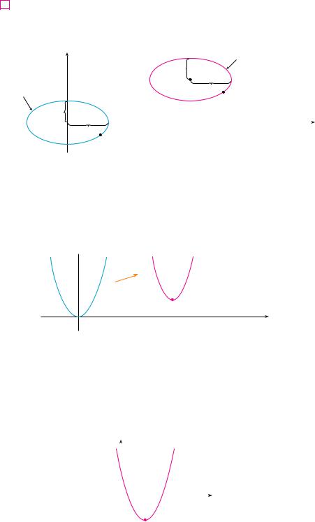
Figure 4 shows the graphs of several parabolas with equations of the form y ax2 for various values of the number a. In each case the vertex, the point where the parabola changes direction, is the origin. We see that the parabola y ax2 opens upward if a 0 and downward if a 0 (as in Figure 5).
y |
|
y |
|
|
0 |
(_x,y) |
(x,y) |
x |
|
0x
(a) y=a≈, a>0 |
(b) y=a≈, a<0 |
FIGURE 5
Notice that if x, y satisfies y ax2, then so does x, y . This corresponds to the geometric fact that if the right half of the graph is reflected about the y-axis, then the left half of the graph is obtained. We say that the graph is symmetric with respect to the y-axis.
The graph of an equation is symmetric with respect to the y-axis if the equation is unchanged when x is replaced by x.
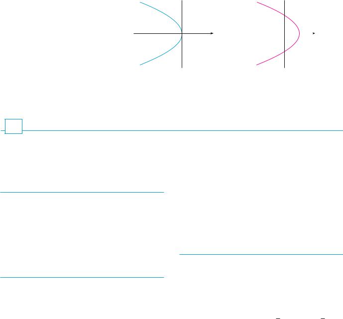
If we interchange x and y in the equation y ax2, the result is x ay2, which also represents a parabola. (Interchanging x and y amounts to reflecting about the diagonal line y x.) The parabola x ay2 opens to the right if a 0 and to the left if a 0. (See

APPENDIX C GRAPHS OF SECOND-DEGREE EQUATIONS |||| A19
Figure 6.) This time the parabola is symmetric with respect to the x-axis because if x, y satisfies x ay2, then so does x, y .
y |
y |
0 |
x |
0 x |
FIGURE 6 |
(a) x=a¥, a>0 |
(b) x=a¥, a<0 |
y
2
(4,2)
x=¥
1
y=x-2
0 |
4 x |
 (1,_1)
FIGURE 7
The graph of an equation is symmetric with respect to the x-axis if the equation is unchanged when y is replaced by y.
EXAMPLE 4 Sketch the region bounded by the parabola x y2 and the line y x 2.
SOLUTION First we find the points of intersection by solving the two equations. Substituting x y 2 into the equation x y2, we get y 2 y2, which gives
0 y2 y 2 y 2 y 1
so y 2 or 1. Thus the points of intersection are 4, 2 and 1, 1 , and we draw
the line y x 2 passing through these points. We then sketch the parabola x y2 by referring to Figure 6(a) and having the parabola pass through 4, 2 and 1, 1 . The region bounded by x y2 and y x 2 means the finite region whose boundaries are
these curves. It is sketched in Figure 7. |
|
|
|
M |
||
ELLIPSES |
|
|
|
|
|
|
The curve with equation |
|
|
|
|
|
|
|
|
|
|
|
|
|
|
|
x2 |
|
y2 |
|
|
2 |
|
|
|
|
1 |
|
a2 |
b2 |
|||||
|
|
|
|
|
|
|
y
(0,b)
(_a,0) |
(a,0) |
0 x
(0,_b)
FIGURE 8
≈ ¥ a@+b@=1
where a and b are positive numbers, is called an ellipse in standard position. (Geometric properties of ellipses are discussed in Section 10.5.) Observe that Equation 2 is unchanged if x is replaced by x or y is replaced by y, so the ellipse is symmetric with respect to both axes. As a further aid to sketching the ellipse, we find its intercepts.
The x-intercepts of a graph are the x-coordinates of the points where the graph intersects the x-axis. They are found by setting y 0 in the equation of the graph.
The y-intercepts are the y-coordinates of the points where the graph intersects the y-axis. They are found by setting x 0 in its equation.
If we set y 0 in Equation 2, we get x2 a2 and so the x-intercepts are a. Setting x 0, we get y2 b2, so the y-intercepts are b. Using this information, together with symmetry, we sketch the ellipse in Figure 8. If a b, the ellipse is a circle with radius a.
A20 |||| APPENDIX C GRAPHS OF SECOND-DEGREE EQUATIONS
FIGURE 9
9≈+16¥=144
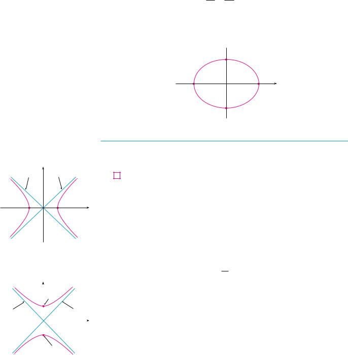
EXAMPLE 5 Sketch the graph of 9x2 16y2 144.
SOLUTION We divide both sides of the equation by 144:
x2 y2 1 16 9
The equation is now in the standard form for an ellipse (2), so we have a2 16, b2 9, a 4, and b 3. The x-intercepts are 4; the y-intercepts are 3. The graph is sketched in Figure 9.
y
(0,3)
(_4,0) |
(4,0) |
0 |
x |
(0,_3)
M
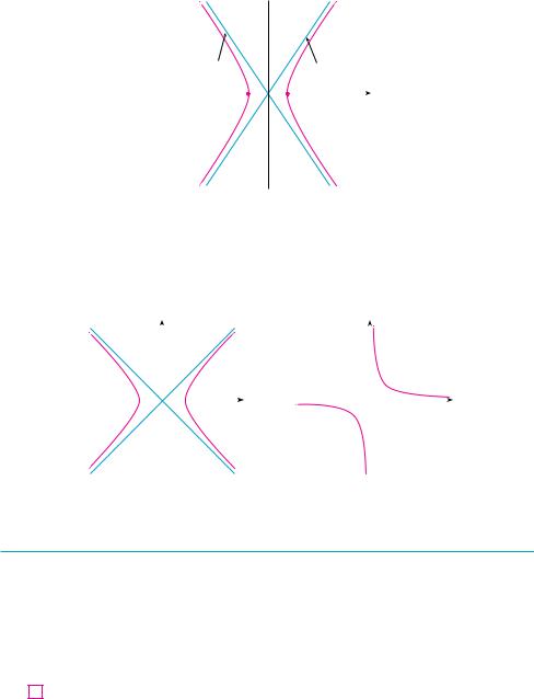
HYPERBOLAS
The curve with equation
y=_ b x |
y |
|
y=b x |
|
|
a |
a |
|
(_a,0) |
(a,0) |
x |
|
0 |
|
FIGURE 10
|
|
≈ |
¥ |
|
|
|
The hyperbola |
|
- |
|
=1 |
|
|
a@ |
b@ |
|||||
|
|
y |
(0,a) |
|
|
|
|
|
|
|
|
||
|
y=_ a x |
|
|
|
y=a x |
|
|
b |
|
|
|
b |
|
|
|
|
|
|
|
|
|
|
0 |
|
|
x |
|
|
|
|
|
|
|
|
|
|
|
(0,_a) |
|||
FIGURE 11 |
|
|
|
|
|
|
|
|
|
|
|
||
The hyperbola |
¥ |
- |
≈ |
=1 |
|
|
a@ |
b@ |
|
||||
|
|
x2 |
|
y2 |
|
3 |
|
|
|
|
1 |
a2 |
b2 |
||||
|
|
|
|
|
|
is called a hyperbola in standard position. Again, Equation 3 is unchanged when x is replaced by x or y is replaced by y, so the hyperbola is symmetric with respect to both axes. To find the x-intercepts we set y 0 and obtain x2 a2 and x a. However, if we put x 0 in Equation 3, we get y2 b2, which is impossible, so there is no y-inter- cept. In fact, from Equation 3 we obtain
x2 |
|
y2 |
|
|
1 |
|
1 |
a2 |
b2 |
||
which shows that x2 a2 and so x sx2 a. Therefore we have x a or x a. This means that the hyperbola consists of two parts, called its branches. It is sketched in Figure 10.
In drawing a hyperbola it is useful to draw first its asymptotes, which are the lines y b a x and y b a x shown in Figure 10. Both branches of the hyperbola approach the asymptotes; that is, they come arbitrarily close to the asymptotes. This involves the idea of a limit, which is discussed in Chapter 2. (See also Exercise 69 in Section 4.5.)
By interchanging the roles of x and y we get an equation of the form
y2 |
|
x2 |
1 |
a2 |
b2 |
which also represents a hyperbola and is sketched in Figure 11.
APPENDIX C GRAPHS OF SECOND-DEGREE EQUATIONS |||| A21
EXAMPLE 6 Sketch the curve 9x2 4y2 36.
SOLUTION Dividing both sides by 36, we obtain
x2 |
y |
2 |
1 |
|
|
|
|
|
|
4 |
9 |
|
||
|
|
|
||
which is the standard form of the equation of a hyperbola (Equation 3). Since a2 4, the x-intercepts are 2. Since b2 9, we have b 3 and the asymptotes are y (32 )x. The hyperbola is sketched in Figure 12.
y
y=_ |
3 x |
y= |
3 x |
|
|
2 |
|
2 |
|
|
|
|
|
|
|
(_2,0) |
(2,0) |
x |
|
|
|
0 |
|
|
FIGURE 12
The hyperbola 9≈-4¥=36
M
If b a, a hyperbola has the equation x2 y2 a2 (or y2 x2 a2) and is called an equilateral hyperbola [see Figure 13(a)]. Its asymptotes are y x, which are perpendicular. If an equilateral hyperbola is rotated by 45 , the asymptotes become the x- and y-axes, and it can be shown that the new equation of the hyperbola is xy k, where k is a constant [see Figure 13(b)].
|
y=_x |
y |
|
y=x |
y |
|
|
|
|
|
|
|
|||||
|
|
|
|
|
|
|||
|
|
|
|
|
|
|
|
|
|
|
|
|
x |
|
|
|
|
|
|
0 |
0 |
|
x |
|||
|
|
|
|
|
|
|
|
|
FIGURE 13 |
|
|
|
|
|
|
|
|
(a) ≈-¥=a@ |
(b) xy=k (k>0) |
|
||||||
Equilateral hyperbolas |
|
|||||||
SHIFTED CONICS
Recall that an equation of the circle with center the origin and radius r is x2 y2 r2, but if the center is the point h, k , then the equation of the circle becomes
x h 2 y k 2 r2
Similarly, if we take the ellipse with equation
|
|
x2 |
|
y2 |
|
4 |
|
|
|
|
1 |
a2 |
b2 |
||||
|
|
|
|
|
|
A22 |||| APPENDIX C GRAPHS OF SECOND-DEGREE EQUATIONS
and translate it (shift it) so that its center is the point h, k , then its equation becomes
5 |
|
|
|
|
|
x h 2 |
|
|
y k 2 |
|
1 |
|
||||||||||
|
|
|
|
|
a2 |
b2 |
||||||||||||||||
|
|
|
|
|
|
|
|
|
|
|
|
|
|
|
|
|
|
|
||||
(See Figure 14.) |
|
|
|
|
|
|
|
|
|
|
|
|
|
|
|
|
|
|||||
|
|
|
|
|
|
|
|
|
|
|
|
|
|
|
|
|
||||||
|
|
|
|
|
y |
|
|
|
|
|
|
|
|
|
|
|
|
(x-h)@ |
+ |
(y-k)@ |
=1 |
|
|
|
|
|
|
|
|
|
|
|
|
|
b |
|
|
a@ |
b@ |
||||||
|
|
|
|
|
|
|
|
|
|
|
|
(h,k) |
||||||||||
|
|
≈ |
|
¥ |
|
|
|
|
|
|
|
|
|
|
|
|
|
|
|
|
|
|
|
|
+ |
=1 |
|
|
|
|
|
|
|
|
a |
||||||||||
|
|
a@ |
b@ |
|
|
|
|
|
|
|
|
|||||||||||
|
|
|
|
|
|
|
|
|
|
|
|
|
(x,y) |
|||||||||
|
|
|
|
|
b |
|
|
|
|
|
|
|
|
|
k |
|||||||
|
|
|
|
|
|
|
|
|
|
|
|
|
|
|
|
|
|
|
|
|
|
|
|
|
|
|
|
(0, 0) |
a |
|
|
|
|
|
|
|
|
|
|
|
x |
||||
|
|
|
|
|
|
|
|
|
|
|
|
|
|
|
|
|
|
|
||||
|
|
|
|
|
|
|
(x-h,y-k) |
|
|
h |
|
|
|
|
|
|
|
|
|
|||
FIGURE 14
Notice that in shifting the ellipse, we replaced x by x h and y by y k in Equation 4 to obtain Equation 5. We use the same procedure to shift the parabola y ax2 so that its vertex (the origin) becomes the point h, k as in Figure 15. Replacing x by x h and y by y k, we see that the new equation is
y k a x h 2 or y a x h 2 k
y
y=a(x-h)@+k
y=a≈
(h,k)
0x
FIGURE 15
EXAMPLE 7 Sketch the graph of the equation y 2x2 4x 1.
SOLUTION First we complete the square:
y 2 x2 2x 1 2 x 1 2 1
In this form we see that the equation represents the parabola obtained by shifting
y 2x2 so that its vertex is at the point 1, 1 . The graph is sketched in Figure 16.
|
y |
|
|
|
|
|
|
|
|
|
|
|
|
|
|
|
|
|
|
|
|
|
|
|
|
|
|
1 |
|
|
|
|
|
|
|
|
|
|
|
|
|
|
|
|
|
|
|
|
|
|
|
|
|
||
|
|
|
|
|
|
|
|
|
|
|
|
||
|
|
|
|
|
|
|
|
|
|
|
|
|
|
0 |
|
1 |
2 |
3 x |
|||||||||
FIGURE 16 |
|
|
|
|
|
|
|
|
|
|
|
|
|
y=2≈-4x+1 |
|
(1,_1) |
|
|
|
|
|
|
M |
||||
APPENDIX C GRAPHS OF SECOND-DEGREE EQUATIONS |||| A23
EXAMPLE 8 Sketch the curve x 1 y2.
SOLUTION This time we start with the parabola x y2 (as in Figure 6 with a 1) and shift one unit to the right to get the graph of x 1 y2. (See Figure 17.)
y y
y
|
|
|
|
|
|
0 |
x |
0 |
1 |
x |
|
|
|
|
|
|
|
FIGURE 17 |
(a) x=_¥ |
(b) x=1-¥ |
M |
C EXERCISES
1– 4 Find an equation of a circle that satisfies the given conditions.
1.Center 3, 1 , radius 5
2.Center 2, 8 , radius 10
3.Center at the origin, passes through 4, 7
4.Center 1, 5 , passes through 4, 6
5–9 Show that the equation represents a circle and find the center and radius.
5.x2 y2 4x 10y 13 0
6.x2 y2 6y 2 0
7.x 2 y 2 x 0
8.16x 2 16y 2 8x 32y 1 0
9.2x 2 2y 2 x y 1
10.Under what condition on the coefficients a, b, and c does the equation x 2 y 2 ax by c 0 represent a circle? When that condition is satisfied, find the center and radius of the circle.
11–32 Identify the type of curve and sketch the graph. Do not plot points. Just use the standard graphs given in Figures 5, 6, 8, 10, and 11 and shift if necessary.
11. |
y x 2 |
12. |
y 2 x 2 1 |
13. |
x 2 4y 2 16 |
14. |
x 2y 2 |
15. |
16x 2 25y 2 400 |
16. |
25x 2 4y 2 |
100 |
|
17. |
4x 2 y 2 1 |
18. |
y x 2 |
2 |
|
19. |
x y 2 1 |
20. |
9x 2 25y 2 |
225 |
|
21. |
9y 2 x 2 9 |
22. |
2x 2 5y 2 10 |
||
23. |
x y 4 |
24. |
y x 2 |
2x |
|
25.9 x 1 2 4 y 2 2 36
26.16x 2 9y 2 36y 108
27. |
y x 2 6x 13 |
28. |
x 2 |
y 2 4x 3 0 |
29. |
x 4 y 2 |
30. |
y 2 |
2x 6y 5 0 |
31.x 2 4y 2 6x 5 0
32.4x 2 9y 2 16x 54y 61 0
33–34 Sketch the region bounded by the curves.
33. y 3x, y x 2 |
34. y 4 x 2, x 2y 2 |
|
|
35.Find an equation of the parabola with vertex 1, 1 that passes through the points 1, 3 and 3, 3 .
36.Find an equation of the ellipse with center at the origin that passes through the points (1, 10 s2 3) and ( 2, 5 s5 3).
37– 40 Sketch the graph of the set.
37. |
x, y x 2 y 2 1 |
38. |
x, y x 2 |
y 2 4 |
39. |
x, y y x 2 1 |
40. |
x, y x 2 |
4y 2 4 |
|
|
|
|
|
A24 |||| APPENDIX D TRIGONOMETRY
a
r
¨
r
FIGURE 1
DTRIGONOMETRY
ANGLES
Angles can be measured in degrees or in radians (abbreviated as rad). The angle given by a complete revolution contains 360 , which is the same as 2 rad. Therefore
1 |
|
|
|
|
|
rad 180 |
|
|
|
||
and |
|
|
|
|
|
|
|
|
|
|
|
|
|
|
|
|
|
|
|
|
|
||
2 |
1 rad |
|
180 |
|
|
57.3 |
1 |
|
rad 0.017 rad |
||
|
|
|
180 |
||||||||
|
|
|
|
|
|
||||||
EXAMPLE 1 |
|
|
|
|
|
|
(b) Express 5 4 rad in degrees. |
||||
(a) Find the radian measure of 60 . |
|||||||||||
SOLUTION
(a) From Equation 1 or 2 we see that to convert from degrees to radians we multiply by
6060 180 3 rad
(b)To convert from radians to degrees we multiply by 180 . Thus180. Therefore
4 |
|
4 |
|
|
|
|
|
5 |
rad |
5 |
|
180 |
|
225 |
M |
|
|
|
|
|
|||
In calculus we use radians to measure angles except when otherwise indicated. The following table gives the correspondence between degree and radian measures of some common angles.
Degrees |
0° |
30° |
45° |
60° |
90° |
120° |
135° |
|
150° |
180° |
270° |
360° |
||||||||||||||||
|
|
|
|
|
|
|
|
|
|
|
|
|
|
|
|
|
|
|
|
|
|
|
|
|
|
|
|
|
Radians |
0 |
|
|
|
|
|
|
|
|
2 |
|
3 |
|
|
5 |
|
|
3 |
|
2 |
||||||||
|
|
|
|
|
|
|
|
|
|
|
|
|
|
|
|
|
|
|
|
|
|
|
|
|
||||
6 |
|
4 |
|
3 |
|
2 |
|
3 |
|
4 |
|
|
6 |
|
2 |
|
||||||||||||
|
|
|
|
|
|
|
|
|
|
|
|
|
||||||||||||||||
|
|
|
|
|
|
|
|
|
|
|
|
|
||||||||||||||||
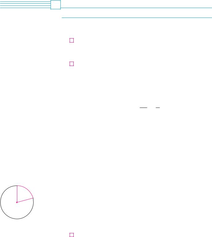
Figure 1 shows a sector of a circle with central angle |
and radius r subtending an arc |
|||||||||||||||||||||||||||
with length a. Since the length of the arc is proportional to the size of the angle, and since the entire circle has circumference 2 r and central angle 2 , we have
|
|
|
|
a |
|
||||
|
2 |
2 r |
|||||||
|
|
||||||||
Solving this equation for and for a, we obtain |
|||||||||
|
|
|
|
|
|
|
|
|
|
3 |
|
a |
|
|
|
|
|
|
a r |
r |
|
||||||||
|
|
|
|
|
|
|
|||
|
|
|
|
|
|
|
|
|
|
Remember that Equations 3 are valid only when
is measured in radians.
r
r
1 |
rad |
r |
|
||
|
|
FIGURE 2
APPENDIX D TRIGONOMETRY |||| A25
In particular, putting a r in Equation 3, we see that an angle of 1 rad is the angle subtended at the center of a circle by an arc equal in length to the radius of the circle (see Figure 2).
EXAMPLE 2
(a)If the radius of a circle is 5 cm, what angle is subtended by an arc of 6 cm?
(b)If a circle has radius 3 cm, what is the length of an arc subtended by a central angle of 3 8 rad?
SOLUTION
(a)Using Equation 3 with a 6 and r 5, we see that the angle is
65 1.2 rad
(b)With r 3 cm and 3 8 rad, the arc length is
|
|
8 |
8 |
|
|
||
a r 3 |
|
3 |
|
|
9 |
cm |
M |
|
|
|
|
||||
The standard position of an angle occurs when we place its vertex at the origin of a coordinate system and its initial side on the positive x-axis as in Figure 3. A positive angle is obtained by rotating the initial side counterclockwise until it coincides with the terminal side. Likewise, negative angles are obtained by clockwise rotation as in Figure 4.
y |
|
y |
|
|
|
|
|
initial side |
|
|
|
|
|
x |
terminal |
|
0 |
¨ |
|
side |
|
|
|
|
¨ |
initial side |
|
terminal side |
|
0x
FIGURE 3 ¨˘0 FIGURE 4 ¨<0
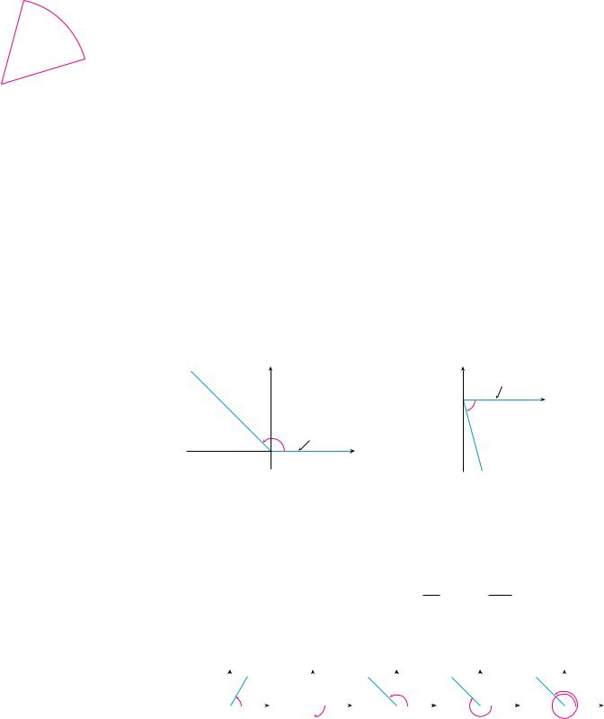
Figure 5 shows several examples of angles in standard position. Notice that different angles can have the same terminal side. For instance, the angles 3 4, 5 4, and 11 4 have the same initial and terminal sides because
and 2
3 |
2 |
5 |
4 |
|
|
4 |
||
rad represents a complete revolution.
3
4
2
11 4
|
y |
|
|
y |
|
|
|
|
y |
|
¨=3π |
y |
|
|
|
|
y |
|
¨=11π4 |
||
|
|
|
|
|
|
|
|
|
|
||||||||||||
|
|
|
|
|
|
|
|
|
|
|
|
|
|
|
|
|
|
||||
|
|
¨=1 |
|
|
|
|
|
|
|
|
4 |
|
|
|
0 |
|
|
|
|
|
|
|
|
|
|
|
|
|
|
|
|
|
|
|
|
|
|
|
|
|
|
||
|
0 |
x |
0 |
|
|
|
x |
0 |
|
x |
|
|
|
|
x |
0 |
|
|
x |
||
FIGURE 5 |
|
|
|
|
¨=_ |
π |
|
|
|
|
|
|
¨=_ |
5π |
|
|
|
|
|||
Angles in standard position |
|
|
|
|
|
2 |
|
|
|
|
|
|
|
|
4 |
|
|
|
|
||
|
|
|
|
|
|
|
|
|
|
|
|
|
|
|
|
|
|
|
|
||
A26 |||| APPENDIX D TRIGONOMETRY |
|
|
|
|
|
|
|
|
|
|||
|
|
|
THE TRIGONOMETRIC FUNCTIONS |
|
|
|
|
|
||||
|
|
|
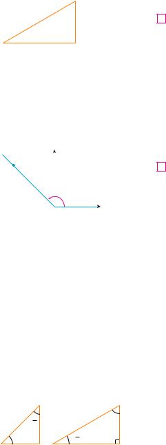
For an acute angle the six trigonometric functions are defined as ratios of lengths of sides |
|||||||||
|
|
|
of a right triangle as follows (see Figure 6). |
|
|
|
|
|
||||
|
|
|
|
|
|
|
|
|
|
|
||
hypotenuse |
4 |
sin |
|
opp |
csc |
|
hyp |
|
||||
|
|
|
|
|
|
|
||||||
|
|
opposite |
|
hyp |
|
opp |
|
|||||
|
|
|
|
|
|
|
|
|
||||
¨ |
|
|
|
cos |
adj |
|
sec |
hyp |
|
|
||
|
|
|
|
|
|
|||||||
adjacent |
|
|
|
|
||||||||
|
hyp |
adj |
||||||||||
|
|
|
|
|
|
|
|
|
||||
FIGURE 6 |
|
|
|
opp |
|
|
|
adj |
|
|
||
|
|
|
|
tan |
|
cot |
|
|
||||
|
|
|
|
adj |
opp |
|||||||
|
|
|
|
|
|
|
|
|
||||
|
|
|
|
|
|
|
|
|
|
|
|
|
This definition doesn’t apply to obtuse or negative angles, so for standard position we let P x, y be any point on the terminal side of distance OP as in Figure 7. Then we define
a general angle inand we let r be the
P(x,y) |
y |
|
|
|
|
5 |
|
|
|
|
|
|
sin |
y |
|
|
|
|
csc |
r |
|
|
|
|
|
|
|
|
|
|
|
|
|||||||||
|
|
|
|
|
|
|
|
|
|
|
|
|
|
|
|
|
|
|
|
|
|
|
|
|
|||||||||||||||||
|
|
|
|
|
|
|
|
|
|
|
|
|
|
|
|
|
|
|
|
|
|
|
|
||||||||||||||||||
|
|
|
|
|
|
|
|
|
|
|
|
|
|
|
|
|
|
|
|
|
|
|
|
|
|
|
|||||||||||||||
|
|
|
|
|
|
|
|
|
|
|
|
|
|
|
|
|
r |
|
|
|
|
|
|
|
|
y |
|
|
|
|
|
|
|
|
|
||||||
r |
|
|
¨ |
|
|
|
|
|
|
|
|
|
cos |
x |
|
|
|
|
|
sec |
r |
|
|
|
|
|
|
|
|
|
|
|
|||||||||
|
|
|
|
|
|
|
|
|
|
|
|
|
|
|
|
|
|
|
|
|
|
|
|
|
|
|
|
||||||||||||||
|
|
|
|
x |
|
|
|
|
|
|
|
r |
|
|
x |
|
|
|
|
|
|
|
|
|
|||||||||||||||||
|
|
|
|
|
|
|
|
|
|
|
|
|
|
|
|
|
|
|
|
|
|
|
|
|
|
|
|
|
|
|
|
|
|||||||||
|
|
|
O |
|
|
|
|
|
|
|
|
|
|
|
|
y |
|
|
|
|
|
|
|
|
|
x |
|
|
|
|
|
|
|
|
|
|
|||||
|
|
|
|
|
|
|
|
|
|
|
|
|
|
|
tan |
|
|
|
cot |
|
|
|
|
|
|
|
|
|
|
||||||||||||
|
|
|
|
|
|
|
|
|
|
|
|
|
|
|
|
|
|
|
|
|
|
|
|
|
|
|
|
||||||||||||||
FIGURE 7 |
|
|
|
|
|
|
|
|
|
|
|
|
x |
|
|
y |
|
|
|
|
|
|
|
|
|
||||||||||||||||
|
|
|
|
|
|
|
|
|
|
|
|
|
|
|
|
|
|
|
|
|
|
|
|
|
|
|
|
|
|
|
|||||||||||
|
|
|
|
|
|
|
|
|
|
|
|
||||||||||||||||||||||||||||||
|
|
|
|
|
|
|
|
Since division by 0 is not defined, tan and sec |
are undefined when x 0 and csc |
||||||||||||||||||||||||||||||||
|
|
|
|
|
|
|
|
and cot are undefined when y 0. Notice that the definitions in (4) and (5) are consis- |
|||||||||||||||||||||||||||||||||
|
|
|
|
|
|
|
|
tent when is an acute angle. |
|
|
|
|
|
|
|
|
|
|
|
|
|
|
|
|
|
|
|
|
|
|
|
|
|
|
|
||||||
|
|
|
|
|
|
|
|
If is a number, the convention is that sin means the sine of the angle whose radian |
|||||||||||||||||||||||||||||||||
|
|
|
|
|
|
|
|
measure is . For example, the expression sin 3 implies that we are dealing with an angle |
|||||||||||||||||||||||||||||||||
|
|
|
|
|
|
|
|
of 3 rad. When finding a calculator approximation to this number, we must remember to |
|||||||||||||||||||||||||||||||||
|
|
|
|
|
|
|
|
set our calculator in radian mode, and then we obtain |
|
|
|
|
|
|
|
|
|
||||||||||||||||||||||||
|
|
|
|
|
|
|
|
|
|
|
|
|
|
|
sin 3 0.14112 |
|
|
|
|
|
|
|
|
|
|||||||||||||||||
|
|
|
|
|
|
|
|
If we want to know the sine of the angle 3 |
we would write sin 3 |
and, with our calculator |
|||||||||||||||||||||||||||||||
|
|
|
|
|
|
|
|
in degree mode, we find that |
|
|
|
|
|
|
|
|
|
|
|
|
|
|
|
|
|
|
|
|
|
|
|
|
|
|
|
||||||
|
|
|
|
|
|
|
|
|
|
|
|
|
|
|
sin 3 |
0.05234 |
|
|
|
|
|
|
|
|
|
||||||||||||||||
|
|
|
|
|
|
|
|
The exact trigonometric ratios for certain angles can be read from the triangles in Fig- |
|||||||||||||||||||||||||||||||||
œ„2 π |
|
|
|
2 |
π |
ure 8. For instance, |
|
|
|
|
|
|
|
|
|
|
|
|
|
|
|
|
|
|
|
|
|
|
|
|
|
|
|
|
|
|
|
|
|
||
4 |
1 |
|
|
|
3 |
1 |
|
|
|
|
|
|
|
|
|
|
|
|
|
|
|
|
|
|
|
|
|
|
|
|
|
s |
|
|
|
|
|||||
4 |
|
|
|
|
|
6 |
|
sin |
|
1 |
sin |
|
1 |
|
|
|
|
|
|
sin |
|
3 |
|
|
|||||||||||||||||
π |
|
|
|
|
π |
|
|
|
|
|
|
|
|
|
|
|
|
|
|
|
|
|
|
|
|
|
|
|
|
|
|
|
|
|
|
|
|
|
|
|
|
1 |
|
|
|
|
|
|
œ„3 |
|
4 |
|
s |
2 |
|
|
|
|
|
|
|
6 |
2 |
|
|
|
|
|
|
|
|
|
3 |
|
|
2 |
|
|
|
||||
|
|
|
|
|
|
|
|
|
|
|
|
1 |
|
|
|
|
|
|
|
|
|
s |
|
|
|
|
|
|
|
|
|
|
|
|
|
|
|
|
|||
FIGURE 8 |
|
|
|
|
|
cos |
|
|
|
cos |
|
3 |
|
|
|
|
|
cos |
|
|
1 |
|
|
|
|
|
|||||||||||||||
|
|
|
|
|
|
|
|
|
|
|
|
|
|
|
|
|
|
|
|
|
|
|
|
|
|||||||||||||||||
|
|
|
|
|
|
|
|
|
4 |
|
s2 |
|
|
|
|
|
|
6 |
2 |
|
|
|
|
|
|
|
3 |
|
|
2 |
|
|
|
|
|
||||||
|
|
|
|
|
|
|
|
tan |
|
1 |
tan |
|
|
1 |
|
|
|
|
|
|
tan |
|
|
|
|
|
|
|
|
|
|||||||||||
|
|
|
|
|
|
|
|
|
|
|
|
|
|
|
|
s |
3 |
|
|
|
|||||||||||||||||||||
|
|
|
|
|
|
|
|
|
|
|
|
|
|
|
|
||||||||||||||||||||||||||
|
|
|
|
|
|
|
|
4 |
6 |
s3 |
|
3 |
|||||||||||||||||||||||||||||
|
|
|
|
|
|
|
|
|
|
|
|
|
|
|
|
|
|
|
|
|
|
|
|
|
|
|
|
|
|
|
|
|
|
||||||||

sin ¨>0 |
y |
all ratios>0 |
0x
tan ¨>0 |
cos ¨>0 |
FIGURE 9
y
P{_1, œ„3} 
2
œ„3
2π π  3 3
3 3
1 0 x
FIGURE 10
5x=œ„„21
¨
2
FIGURE 11
16
x
40°
FIGURE 12
APPENDIX D TRIGONOMETRY |||| A27
The signs of the trigonometric functions for angles in each of the four quadrants can be remembered by means of the rule “All Students Take Calculus” shown in Figure 9.
EXAMPLE 3 Find the exact trigonometric ratios for |
2 3. |
|
|
|
|
|
|
|
|
|
|
|
|
|
|
|
|
|
|
|
||||||||||||||||||||||||||||||||||||||||||||||||||||||||||||
SOLUTION |
From Figure 10 we see that a point on the terminal line for 2 3 is |
|
|
|||||||||||||||||||||||||||||||||||||||||||||||||||||||||||||||||||||||||||||
P( 1, s3 ). Therefore, taking |
|
|
|
|
|
|
|
|
|
|
|
|
|
|
|
|
|
|
|
|
|
|
|
|
|
|
|
|
|
|
|
|
|
|
|
|
|
|
|
|
|
|
|
|
|
|
|
|
|
|
|
|
|
|||||||||||||||||||||||||||
|
|
|
|
|
|
|
|
|
|
|
|
|
|
|
|
|
|
|
|
x 1 |
|
|
|
|
|
y s |
|
|
|
|
|
|
|
|
|
|
|
|
r 2 |
|
|
|
|
|
|
|
|
|
|
|
|
|||||||||||||||||||||||||||||
|
|
|
|
|
|
|
|
|
|
|
|
|
|
|
|
|
|
|
|
|
|
|
|
3 |
|
|
|
|
|
|
|
|
|
|
|
|
|
|
|
|
|
|
|
|
||||||||||||||||||||||||||||||||||||
in the definitions of the trigonometric ratios, we have |
|
|
|
|
|
|
|
|
|
|
|
|
|
|
|
|
|
|
|
|
|
|
||||||||||||||||||||||||||||||||||||||||||||||||||||||||||
|
|
|
|
|
2 |
|
|
|
|
|
|
s |
|
|
|
|
|
|
|
|
|
|
|
|
|
2 |
|
|
|
|
|
|
|
|
|
1 |
|
|
|
|
|
|
|
|
|
|
|
2 |
|
|
|
|
|
|
|
|
|
|
||||||||||||||||||||||
|
|
sin |
|
|
3 |
|
|
|
|
|
|
cos |
|
|
|
|
|
|
|
|
|
|
|
|
|
|
|
|
|
|
tan |
|
s |
|
|
|
|
|
|
|||||||||||||||||||||||||||||||||||||||||
|
|
|
|
|
|
|
|
|
|
|
|
|
|
|
|
|
|
|
|
|
|
|
|
|
|
|
|
|
3 |
|
|
|
|
|||||||||||||||||||||||||||||||||||||||||||||||
|
|
|
|
3 |
|
|
|
|
|
|
|
|
|
|
|
|
3 |
|
|
|
|
|
|
|
|
|
|
|
|
3 |
|
|
|
|
|
|
|
|
||||||||||||||||||||||||||||||||||||||||||
|
|
|
|
|
|
|
|
2 |
|
|
|
|
|
|
|
|
|
|
|
|
2 |
|
|
|
|
|
|
|
|
|
|
|
|
|
|
|
|
|
|
|
|
|
|
|
|
|
|
|
||||||||||||||||||||||||||||||||
|
|
csc |
2 |
|
|
|
|
2 |
|
|
|
|
|
|
|
|
|
|
sec |
2 |
|
|
2 |
|
|
|
|
|
|
|
|
|
cot |
2 |
|
|
1 |
|
|
|
|
|
M |
|||||||||||||||||||||||||||||||||||||
|
|
|
|
|
|
|
|
|
|
|
|
|
|
|
|
|
|
|
|
|
|
|
|
|
|
|
|
|
|
|
|
|
|
|
|
|
|
|
|
|
|
|
|
|
||||||||||||||||||||||||||||||||||||
|
|
|
|
3 |
|
|
s3 |
|
|
|
|
3 |
|
|
|
|
|
|
|
|
3 |
|
|
|
|
s3 |
|
|
||||||||||||||||||||||||||||||||||||||||||||||||||||
|
|
|
|
|
|
|
|
|
|
|
|
|
|
|
|
|
|
|
|
|
|
|
|
|
|
|
|
|
|
|
|
|
|
|
|
|
|
|
|
|
|
|
|
|
|
|
|
|
|
|
|
|
|
|
|
|
||||||||||||||||||||||||
The following table gives some values of sin and |
|
cos |
found by the method of |
|||||||||||||||||||||||||||||||||||||||||||||||||||||||||||||||||||||||||||||
Example 3. |
|
|
|
|
|
|
|
|
|
|
|
|
|
|
|
|
|
|
|
|
|
|
|
|
|
|
|
|
|
|
|
|
|
|
|
|
|
|
|
|
|
|
|
|
|
|
|
|
|
|
|
|
|
|
|
|
|
|
|
|
|
|
|
|
|
|
|
|
|
|
|
|
|
|
|
|
||||
|
|
|
|
|
|
|
|
|
|
|
|
|
|
|
|
|
|
|
|
|
|
|
|
|
|
|
|
|
|
|
|
|
|
|
|
|
|
|
|
|
|
|
|
|
|
|
|
|
|
|
|
|
||||||||||||||||||||||||||||
|
|
0 |
|
|
|
|
|
|
|
|
|
|
|
|
|
|
|
|
|
|
|
|
|
|
|
2 |
|
|
|
|
|
|
3 |
|
|
|
|
|
5 |
|
|
|
|
|
|
|
|
|
3 |
|
2 |
|||||||||||||||||||||||||||||
|
|
|
|
|
|
|
|
|
|
|
|
|
|
|
|
|
|
|
|
|
|
|
|
|
|
|
|
|
|
|
|
|
|
|
|
|
|
|
|
|
|
|
|
|
|
|
|
|
|
|
|
|
|
|
|
|
|
|
|
|
|
|
|
|
|
|
|
|
|
|
|
|
|
|
||||||
|
6 |
|
|
|
|
|
|
4 |
|
|
|
|
|
|
|
|
3 |
|
|
|
2 |
|
|
|
3 |
|
|
|
|
|
|
4 |
|
|
|
|
|
|
6 |
|
|
|
|
|
|
|
|
2 |
||||||||||||||||||||||||||||||||
|
|
|
|
|
|
|
|
|
|
|
|
|
|
|
|
|
|
|
|
|
|
|
|
|
|
|
|
|
|
|
|
|
|
|
|
|
|
|
|
|
|
|
|
|
|
|
|
|||||||||||||||||||||||||||||||||
|
|
|
|
|
|
|
|
|
|
|
|
|
|
|
|
|
|
|
|
|
|
|
|
|
|
|
|
|
|
|
|
|
|
|
|
|
|
|
|
|
|
|
|
|
|
|
|
|
|
|
|
|
|
|
|
|
|
|
|
|
|
|
|
|
|
|
|
|
|
|
|
|
|
|||||||
|
|
|
|
|
1 |
|
|
|
|
1 |
|
|
|
|
|
|
|
|
s |
|
|
|
|
|
|
|
|
|
|
|
|
s |
|
|
|
|
1 |
|
|
|
|
|
|
1 |
|
|
|
|
|
|
|
|
|
|
|
|
|
|
|
|
||||||||||||||||||||
sin |
|
0 |
|
|
|
|
|
|
|
|
|
|
|
|
|
|
3 |
|
|
1 |
|
|
|
|
3 |
|
|
|
|
|
|
|
|
|
|
|
|
0 |
|
|
|
|
1 |
|
0 |
|||||||||||||||||||||||||||||||||||
|
|
|
|
|
|
|
|
|
|
|
|
|
|
|
|
|
|
|
|
|
|
|
|
|
|
|
|
|
|
|
|
|
|
|
|
|
|
|
|
|
|
|
|
|
|
|
|
|
|
|
|
|
|
|
|
|
|
|
|
|
|
|
|
|
|
|
|
|
|
|
||||||||||
|
2 |
|
|
|
|
|
|
|
s2 |
|
2 |
|
|
|
|
2 |
|
|
|
|
|
|
|
|
s2 |
|
|
|
2 |
|
|
|
|
|
|
|
|
|||||||||||||||||||||||||||||||||||||||||||
|
|
|
|
|
|
|
|
|
|
|
|
|
|
|
|
|
|
|
|
|
|
|
|
|
|
|
|
|
|
|
|
|
|
|
|
|
|
|
|
|
|
|
|
|
|
|
|
|||||||||||||||||||||||||||||||||
|
|
1 |
|
s |
|
|
|
|
|
1 |
|
|
|
|
|
|
|
|
1 |
|
|
|
|
|
|
|
|
|
|
1 |
|
|
|
|
|
|
1 |
|
|
|
|
|
|
s |
|
|
|
|
|
|
|
|
|
|
|
|
|
|||||||||||||||||||||||
cos |
3 |
|
|
|
|
|
|
|
|
|
|
|
0 |
|
|
|
|
|
|
|
|
|
|
|
3 |
|
|
1 |
|
|
|
|
0 |
|
1 |
|||||||||||||||||||||||||||||||||||||||||||||
|
|
|
|
|
|
|
|
|
|
|
|
|
|
|
|
|
|
|
|
|
|
|
|
|
|
|
|
|
|
|
|
|
|
|
|
|
|
|
|
|
|
|
|
|
|
|
|
|
|
|
|
|||||||||||||||||||||||||||||
|
|
|
|
|
2 |
|
|
|
|
|
|
|
s2 |
|
2 |
|
|
|
|
|
|
|
|
2 |
|
|
|
|
|
|
|
|
s2 |
|
|
|
2 |
|
|
|
|
|
|
|
|
|
|
|
|
|
|
|||||||||||||||||||||||||||||
EXAMPLE 4 If cos |
|
|
|
52 and 0 |
2, find the other five trigonometric functions |
|||||||||||||||||||||||||||||||||||||||||||||||||||||||||||||||||||||||||||
of . |
|
|
|
|
|
|
|
|
|
|
|
|
|
|
|
|
|
|
|
|
|
|
|
|
|
|
|
|
|
|
|
|
|
|
|
|
|
|
|
|
|
|
|
|
|
|
|
|
|
|
|
|
|
|
|
|
|
|
|
|
|
|
|
|
|
|
|
|
|
|
|
|
|
|
|
|
|
|
|
|
SOLUTION |
Since cos |
|
52 , we can label the hypotenuse as having length 5 and the |
|
|
|||||||||||||||||||||||||||||||||||||||||||||||||||||||||||||||||||||||||||
adjacent side as having length 2 in Figure 11. If the opposite side has length x, then the Pythagorean Theorem gives x2 4 25 and so x2 21, x s21. We can now use the diagram to write the other five trigonometric functions:
|
sin |
s21 |
|
|
|
|
tan |
s21 |
|
|
|
|
|
|
|||||||
|
|
|
|
|
2 |
|
|
|
|
|
|||||||||||
|
5 |
|
|
|
|
|
|
|
|
|
|
|
|
|
|
||||||
csc |
5 |
|
|
|
|
sec |
|
5 |
|
cot |
2 |
|
|
M |
|||||||
|
|
|
|
|
|
|
|
|
|
|
|||||||||||
|
s21 |
|
|
2 |
|
|
|
|
s21 |
|
|||||||||||
EXAMPLE 5 Use a calculator to approximate the value of x in Figure 12. |
|
||||||||||||||||||||
SOLUTION From the diagram we see that |
|
|
|
|
|
|
|
|
|
|
|
|
|
|
|
||||||
|
|
|
|
|
tan 40 |
|
16 |
|
|
|
|
|
|
|
|
||||||
|
x |
|
|
|
|
|
|
|
|||||||||||||
|
|
|
|
|
|
|
|
|
|
|
|
|
|
|
|
|
|
|
|||
Therefore |
|
|
|
x |
|
16 |
|
19.07 |
|
|
|
|
|
|
M |
||||||
|
tan 40 |
|
|
|
|
|
|
|
|||||||||||||
|
|
|
|
|
|
|
|
|
|
|
|
|
|
|
|
|
|
|
|
||
A28 |||| APPENDIX D TRIGONOMETRY
TRIGONOMETRIC IDENTITIES
N Odd functions and even functions are discussed in Section 1.1.
A trigonometric identity is a relationship among the trigonometric functions. The most elementary are the following, which are immediate consequences of the definitions of the trigonometric functions.
6 |
csc |
1 |
|
|
sec |
|
1 |
|
cot |
|
1 |
|
|
sin |
|
|
cos |
|
tan |
|
|
||||||
|
|
|
|
|
|
|
|
|
|||||
|
|
tan |
|
sin |
|
cot |
|
cos |
|
|
|
|
|
|
cos |
|
sin |
|
|
|
|
||||||
|
|
|
|
|
|
|
|
|
|
|
|
||
|
|
|
|
|
|
|
|
|
|
|
|
|
|
For the next identity we refer back to Figure 7. The distance formula (or, equivalently, the Pythagorean Theorem) tells us that x2 y2 r2. Therefore
sin2 cos2 |
y2 |
|
x2 |
|
x2 y2 |
|
r2 |
1 |
|
r2 |
r2 |
r2 |
r2 |
||||||
|
|
|
|
|
We have therefore proved one of the most useful of all trigonometric identities:
7 |
sin2 cos2 1 |
|
|
If we now divide both sides of Equation 7 by cos2 and use Equations 6, we get
8 |
tan2 1 sec2 |
|
|
Similarly, if we divide both sides of Equation 7 by sin2 , we get
9 |
1 cot2 csc2 |
|
The identities |
|
|
|
|
|
|
|
|
10 a |
sin sin |
|
10 b |
cos cos |
|
|
|
|
show that sin is an odd function and cos is an even function. They are easily proved by drawing a diagram showing and in standard position (see Exercise 39).
Since the angles and 2 have the same terminal side, we have
11 |
sin 2 sin |
cos 2 cos |
|
|
|
These identities show that the sine and cosine functions are periodic with period 2 . The remaining trigonometric identities are all consequences of two basic identities
called the addition formulas:

|
|
APPENDIX D TRIGONOMETRY |||| A29 |
|
|
|
|
|
|
|
sin x y sin x cos y cos x sin y |
|
1 2 a |
|||
|
|
cos x y cos x cos y sin x sin y |
|
1 2 b |
|||
|
|
|
|
The proofs of these addition formulas are outlined in Exercises 85, 86, and 87.
By substituting y for y in Equations 12a and 12b and using Equations 10a and 10b, we obtain the following subtraction formulas:
1 3 a |
sin x y sin x cos y cos x sin y |
1 3 b |
cos x y cos x cos y sin x sin y |
|
|
Then, by dividing the formulas in Equations 12 or Equations 13, we obtain the corresponding formulas for tan x y :
1 4 a |
tan x y |
tan x tan y |
|
1 tan x tan y |
|
||
|
|
|
|
1 4 b |
tan x y |
tan x tan y |
|
1 tan x tan y |
|
||
|
|
|
|
|
|
|
|
If we put y x in the addition formulas (12), we get the double-angle formulas:
|
|
sin 2x 2 sin x cos x |
15 a |
||
|
|
cos 2x cos2x sin2x |
15 b |
||
|
|
|
Then, by using the identity sin2x cos2x 1, we obtain the following alternate forms of the double-angle formulas for cos 2x:
16 a |
cos 2x 2 cos2x 1 |
16 b |
cos 2x 1 2 sin2x |
|
|
If we now solve these equations for cos2x and sin2x, we get the following half-angle formulas, which are useful in integral calculus:
1 7 a |
cos2x |
1 cos 2x |
|
|
|
|
|||
|
2 |
|
||
1 7 b |
sin2x |
|
1 cos 2x |
|
|
|
|
||
|
2 |
|
||
|
|
|
|
|
Finally, we state the product formulas, which can be deduced from Equations 12 and 13:

A30 |||| APPENDIX D TRIGONOMETRY
1 8 a |
sin x cos y 21 |
sin x y sin x y |
1 8 b |
cos x cos y 21 |
cos x y cos x y |
1 8 c |
sin x sin y 21 |
cos x y cos x y |
|
|
|
There are many other trigonometric identities, but those we have stated are the ones used most often in calculus. If you forget any of them, remember that they can all be deduced from Equations 12a and 12b.
EXAMPLE 6 Find all values of x in the interval 0, 2 such that sin x sin 2x.
SOLUTION Using the double-angle formula (15a), we rewrite the given equation as
sin x 2 sin x cos x |
or |
sin x 1 2 cos x 0 |
|||||
Therefore, there are two possibilities: |
|
|
|
|
|
|
|
sin x 0 |
or |
1 2 cos x |
0 |
|
|
|
|
x 0, , 2 |
or |
cos x |
21 |
|
|
|
|
|
|
|
|
5 |
|
||
x |
or |
x |
|
|
, |
|
|
3 |
|
||||||
|
|
|
3 |
|
|||
The given equation has five solutions: 0, |
3, |
, 5 3, and 2 . |
|
|
|
||
GRAPHS OF THE TRIGONOMETRIC FUNCTIONS
M
The graph of the function f x sin x, shown in Figure 13(a), is obtained by plotting points for 0 x 2 and then using the periodic nature of the function (from Equation 11) to complete the graph. Notice that the zeros of the sine function occur at the
|
y |
|
|
|
|
_ |
π 1 |
|
|
3π |
|
2 |
|
|
2 |
|
|
_π |
0 |
π |
π |
x |
3π |
_1 |
2 |
2π 5π |
|||
|
|
2 |
|
(a) ƒ=sin x
|
y |
|
|
|
|
_π |
1 |
|
π |
|
3π |
|
|
|
|||
_ |
π |
0 π |
3π |
2π 5π |
x |
2 _1 |
2 |
2 |
2 |
|
FIGURE 13 |
(b) ©=cos x |

APPENDIX D TRIGONOMETRY |||| A31
integer multiples of , that is,
sin x 0
Because of the identity
whenever x n
cos x sin x
,
2
n an integer
(which can be verified using Equation 12a), the graph of cosine is obtained by shifting the graph of sine by an amount 2 to the left [see Figure 13(b)]. Note that for both the sine and cosine functions the domain is , and the range is the closed interval 1, 1 . Thus, for all values of x, we have
1 sin x 1 1 cos x 1
The graphs of the remaining four trigonometric functions are shown in Figure 14 and their domains are indicated there. Notice that tangent and cotangent have range , , whereas cosecant and secant have range , 1 1, . All four functions are periodic: tangent and cotangent have period , whereas cosecant and secant have period 2 .
y y
y
_π |
|
1 |
|
|
|
|
|
|
|
0 |
|
|
|
|
|
|
|
_ |
π |
π π 3π x |
_π |
_ |
π 0 |
π π |
3π x |
|
2 |
_1 2 |
2 |
|
2 |
2 |
2 |
||
|
|
|
||||||
|
|
|
|
|
(a) y=tan x |
|
|
|
|
|
|
|
|
(b) y=cot x |
|
|
|
|
|||||||||
|
|
|
|
y |
|
|
|
|
|
|
y=sin x |
|
|
|
|
y |
|
|
y=cos x |
|
|||||||
|
|
|
|
|
|
|
|
|
|
|
|
|
|
|
|
|
|
|
|
|
|||||||
|
π |
1 |
|
|
|
|
|
|
|
3π |
|
|
|
|
1 |
|
|
|
|
|
|
|
|||||
_ |
|
|
|
|
|
|
|
_π _ |
π |
|
|
|
|
|
|
3π |
|
||||||||||
|
|
|
|
|
|
|
|
|
|
|
|
||||||||||||||||
|
2 |
0 |
|
|
|
|
|
|
|
2 |
|
2 |
0 |
|
|
|
2 |
|
|||||||||
|
|
|
|
|
|
|
π π |
|
|
|
x |
|
|
|
|
|
|
|
π |
π |
x |
||||||
|
|
|
|
|
|
|
_1 |
2 |
|
|
|
|
|
|
|
|
|
_1 |
|
|
2 |
|
|
|
|
||
|
|
|
|
|
|
|
|
|
|
|
|
|
|
|
|
|
|
|
|
|
|||||||
|
|
|
|
|
|
|
|
|
|
|
|
|
|
|
|
|
|
|
|
|
|
|
|
|
|
|
|
FIGURE 14 |
(c) y=csc x |
(d) y=sec x |
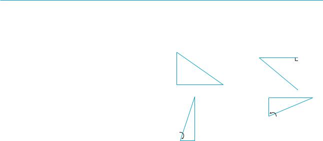
A32 |||| APPENDIX D TRIGONOMETRY
|
|
|
D |
|
EXERCISES |
|
|
|
|
|
|
|
|
|
|
|
|
|
|||||||
1–6 Convert from degrees to radians. |
|
|
|
|||||||||
1. |
210 |
|
2. |
300 |
|
3. |
9 |
|
||||
4. |
315 |
5. |
900 |
|
6. |
36 |
|
|||||
|
|
|
|
|
|
|
|
|
|
|||
7–12 Convert from radians to degrees. |
|
|
|
|||||||||
7. |
4 |
|
|
8. |
|
7 |
|
9. |
5 |
|
||
|
|
|
|
12 |
|
|||||||
|
|
|
|
|
|
|
2 |
|
|
|
||
10. |
8 |
|
|
11. |
|
3 |
|
12. |
5 |
|
||
3 |
|
|
|
|
||||||||
|
|
|
|
|
|
8 |
|
|
|
|
||
|
|
|
|
|
|
|
|
|
|
|
|
|
13.Find the length of a circular arc subtended by an angle of12 rad if the radius of the circle is 36 cm.
14.If a circle has radius 10 cm, find the length of the arc subtended by a central angle of 72 .
15.A circle has radius 1.5 m. What angle is subtended at the center of the circle by an arc 1 m long?
16.Find the radius of a circular sector with angle 3 4 and arc length 6 cm.
17–22 Draw, in standard position, the angle whose measure is given.
17. |
315 |
18. |
150 |
19. |
|
3 |
rad |
||
|
|||||||||
|
|
|
|
|
|
4 |
|
||
20. |
7 |
rad |
21. |
2 rad |
22. |
3 rad |
|||
3 |
|||||||||
|
|
|
|
|
|
|
|
||
|
|
|
|
|
|
|
|
|
|
23–28 Find the exact trigonometric ratios for the angle whose radian measure is given.
|
3 |
|
4 |
9 |
|
|
||
23. |
|
|
24. |
|
25. |
|
|
|
4 |
|
|
|
|
|
|||
|
|
3 |
2 |
|
|
|||
|
5 |
5 |
11 |
|
||||
26. |
27. |
|
28. |
|
|
|
||
|
|
|
|
|||||
|
|
|
6 |
4 |
|
|
||
|
|
|
|
|
|
|
|
|
29–34 Find the remaining trigonometric ratios.
29. |
sin |
3 |
, |
|
0 |
|
|
|
|
|
|
|
|
|
|
||||
|
|
|
|
|
|
|
|
|
|
|
|
|
|||||||
5 |
|
2 |
|
|
|
|
|
|
|||||||||||
30. |
tan |
2, |
|
0 |
|
|
|
|
|
|
|
|
|||||||
|
|
|
|
|
|
|
|
|
|||||||||||
|
2 |
|
|
|
|
|
|
||||||||||||
31. |
sec 1.5, |
|
|
|
|
|
|
||||||||||||
|
2 |
|
|||||||||||||||||
32. |
cos x |
1 |
|
, |
x |
3 |
|
||||||||||||
|
|
|
|
|
|
||||||||||||||
3 |
|
2 |
|
|
|||||||||||||||
33. |
cot |
3, |
|
|
|
|
2 |
|
|
|
|||||||||
34. csc |
4 |
, |
3 |
2 |
3 |
2 |
|||
|
|
|
|
|
35–38 Find, correct to five decimal places, the length of the side labeled x.
35. |
36. |
x |
||
|
|
|
10 cm |
40° |
|
|
|
|
|
|
x |
25 cm |
||
|
|
|
35° |
|
|
|
|
|
|
|
|
|
|
|
37. |
|
|
|
|
|
|
|
|
|
|
|
|
|
|
|
38. |
|
|
|
|
|
|
|
|
|
|
|
|
|
|
|
|
|
|
|||
|
|
|
|
|
|
|
|
|
|
|
|
|
|
|
|
22cm |
||
|
|
|
|
|
|
|
|
|
|
|
|
|
|
|
|
|
|
x |
|
|
|
|
|
|
|
|
|
x |
|
|
|
|
|
|
|
|
3π |
|
|
|
|
|
|
|
|
|
|
|
|
|
|
|
8 |
|||
|
|
|
|
|
|
|
|
|
|
|
|
|
|
|
|
|||
|
2π |
|
|
|
|
|
|
|
|
|
|
|
|
|
|
|
|
|
|
5 |
|
|
|
|
|
|
|
|
|
|
|
|
|
|
|
|
|
|
|
|
|
|
|
|
|
|
|
|
|
|
|
|
|
|||
|
|
8cm |
|
|
|
|
|
|
|
|
|
|
|
|
||||
|
|
|
|
|
|
|
|
|
|
|
|
|
|
|||||
39– 41 Prove each equation. |
|
|
|
|
||||||||||||||
39. |
(a) Equation 10a |
|
|
|
|
(b) |
Equation 10b |
|||||||||||
40. |
(a) Equation 14a |
|
|
|
|
(b) |
Equation 14b |
|||||||||||
41. |
(a) Equation 18a |
|
|
|
|
(b) |
Equation 18b |
|||||||||||
|
(c) Equation 18c |
|
|
|
|
|
|
|
|
|||||||||
|
|
|
|
|
|
|
|
|
|
|
|
|
|
|
||||
42–58 Prove the identity. |
|
|
|
|
|
|
||||||||||||
|
|
2 |
|
|
|
|
|
|
|
|
|
|
|
|
|
|
|
|
42. |
cos |
|
|
x sin x |
|
|
|
|
|
|
||||||||
|
|
|
|
|
|
|
|
|
||||||||||
|
2 |
|
|
|
|
|
|
|
|
|
|
|
|
|
|
|
||
43. |
sin |
|
|
x cos x |
|
|
|
44. sin x sin x |
||||||||||
|
|
|
|
|
|
|||||||||||||
45. |
sin |
|
cot cos |
|
|
|
46. sin x cos x 2 1 sin 2x |
|||||||||||
47. |
sec y cos y tan y sin y |
|
|
|
||||||||||||||
48. |
tan2 |
sin2 tan2 sin2 |
|
|
|
|||||||||||||
49. |
cot2 |
sec2 tan2 csc2 |
||||||||||||||||
50. |
2 csc 2t sec t csc t |
|
|
|
|
|
|
|||||||||||
51. |
tan 2 |
|
|
|
2 tan |
|
|
|
|
|
|
|
|
|||||
1 tan2 |
|
|
|
|
|
|
||||||||||||
52. |
|
1 |
|
|
|
|
|
|
|
1 |
|
|
|
2 sec2 |
||||
1 sin |
|
1 sin |
|
|
||||||||||||||
|
|
|
|
|
|
|
|
|
||||||||||
53.sin x sin 2x cos x cos 2x cos x
54.sin2x sin2 y sin x y sin x y
55. |
|
sin |
csc cot |
|
cos |
||
1 |
|
||

56. |
tan x tan y |
sin x y |
|
|
cos x cos y |
||||
|
|
|||
57. |
sin 3 sin 2 sin 2 cos |
|||
58. |
cos 3 4 cos3 3 cos |
|||
|
|
|
|
|
59–64 If sin x 13 and sec y 54, where x and y lie between 0 and
2, evaluate the expression. |
|
|
|
59. |
sin x y |
60. |
cos x y |
61. |
cos x y |
62. |
sin x y |
63. |
sin 2y |
64. |
cos 2y |
|
|
|
|
65–72 Find all values of x in the interval 0, 2 that satisfy the equation.
65. |
2 cos x 1 0 |
66. |
3 cot2x 1 |
67. |
2 sin2x 1 |
68. |
tan x 1 |
69. |
sin 2x cos x |
70. |
2 cos x sin 2x 0 |
71. |
sin x tan x |
72. |
2 cos 2x 3 cos x |
|
|
|
|
73–76 Find all values of x in the interval 0, 2 that satisfy the inequality.
73. |
sin x 21 |
74. |
2 cos x 1 0 |
75. |
1 tan x 1 |
76. |
sin x cos x |
|
|
|
|
77– 82 Graph the function by starting with the graphs in Figures 13 and 14 and applying the transformations of Section 1.3 where
appropriate. |
|
|
|
|
|
|
|
|
|
|
|
|
|||
|
|
|
|
|
|
|
|
|
|
|
|
|
|
|
|
77. |
y cos x |
|
|
|
|
|
78. |
y tan 2x |
|
|
|||||
|
|
|
|
|
|||||||||||
|
|
|
|
|
|
3 |
|
|
|
|
|
||||
79. |
y |
1 |
tan |
x |
|
|
80. |
y 1 sec x |
|
|
|||||
|
2 |
|
|
||||||||||||
|
3 |
|
|
|
|
|
y 2 sin x |
|
|
||||||
81. |
y sin x |
|
|
|
|
|
|
82. |
|
||||||
|
|
|
|
|
|
|
|||||||||
|
|
|
|
|
|
4 |
|||||||||
|
|
|
|
|
|
|
|
||||||||
83. |
Prove the Law of Cosines: If a triangle has sides with lengths |
||||||||||||||
|
a, b, and c, and |
is the angle between the sides with lengths a |
|||||||||||||
|
and b, then |
|
|
|
|
|
|
|
|
|
|
||||
|
|
|
|
|
|
|
|
|
c 2 a 2 b 2 2ab cos |
|
|
||||
|
|
|
|
|
|
|
|
|
|
y |
|
P(x,y) |
|
|
|
|
|
|
|
|
|
|
|
|
|
|
|
|
|
|
|
bc
|
|
¨ |
|
|
|
|
|
|
|
0 |
|
|
|
(a,0) |
|
x |
|
[Hint: Introduce a coordinate system so that |
is in standard |
|||||||
APPENDIX D TRIGONOMETRY |
|||| A33 |
|
position as in the figure. Express x and y in terms of |
|
and then |
|
||
use the distance formula to compute c.]
84.In order to find the distance AB across a small inlet, a point C is located as in the figure and the following measurements were recorded:
C 103 AC 820 m BC 910 m
Use the Law of Cosines from Exercise 83 to find the required distance.
A
C
B
85. Use the figure to prove the subtraction formula
cos cos cos sin sin
[Hint: Compute c2 in two ways (using the Law of Cosines from Exercise 83 and also using the distance formula) and compare the two expressions.]
y |
|
|
A(cos å,sin å) |
|||
|
||||||
|
|
|
||||
|
|
|
|
c |
||
|
|
1 |
1 |
|
B(cos ∫,sin ∫) |
|
|
|
|
|
|
|
|
|
|
å |
∫ |
|
|
x |
|
|
|
||||
0 |
|
|
|
|
|
|
|
|
|
|
|
|
|
86.Use the formula in Exercise 85 to prove the addition formula for cosine (12b).
87.Use the addition formula for cosine and the identities
2 |
|
|
2 |
|
|
|
|
|
|
|
|
cos |
|
sin |
sin |
|
cos |
to prove the subtraction formula for the sine function.
88. Show that the area of a triangle with sides of lengths a and b and with included angle is
A12 ab sin
89.Find the area of triangle ABC, correct to five decimal places, if
AB 10 cm |
BC 3 cm |
ABC 107 |