

- •CONTENTS
- •Preface
- •To the Student
- •Diagnostic Tests
- •1.1 Four Ways to Represent a Function
- •1.2 Mathematical Models: A Catalog of Essential Functions
- •1.3 New Functions from Old Functions
- •1.4 Graphing Calculators and Computers
- •1.6 Inverse Functions and Logarithms
- •Review
- •2.1 The Tangent and Velocity Problems
- •2.2 The Limit of a Function
- •2.3 Calculating Limits Using the Limit Laws
- •2.4 The Precise Definition of a Limit
- •2.5 Continuity
- •2.6 Limits at Infinity; Horizontal Asymptotes
- •2.7 Derivatives and Rates of Change
- •Review
- •3.2 The Product and Quotient Rules
- •3.3 Derivatives of Trigonometric Functions
- •3.4 The Chain Rule
- •3.5 Implicit Differentiation
- •3.6 Derivatives of Logarithmic Functions
- •3.7 Rates of Change in the Natural and Social Sciences
- •3.8 Exponential Growth and Decay
- •3.9 Related Rates
- •3.10 Linear Approximations and Differentials
- •3.11 Hyperbolic Functions
- •Review
- •4.1 Maximum and Minimum Values
- •4.2 The Mean Value Theorem
- •4.3 How Derivatives Affect the Shape of a Graph
- •4.5 Summary of Curve Sketching
- •4.7 Optimization Problems
- •Review
- •5 INTEGRALS
- •5.1 Areas and Distances
- •5.2 The Definite Integral
- •5.3 The Fundamental Theorem of Calculus
- •5.4 Indefinite Integrals and the Net Change Theorem
- •5.5 The Substitution Rule
- •6.1 Areas between Curves
- •6.2 Volumes
- •6.3 Volumes by Cylindrical Shells
- •6.4 Work
- •6.5 Average Value of a Function
- •Review
- •7.1 Integration by Parts
- •7.2 Trigonometric Integrals
- •7.3 Trigonometric Substitution
- •7.4 Integration of Rational Functions by Partial Fractions
- •7.5 Strategy for Integration
- •7.6 Integration Using Tables and Computer Algebra Systems
- •7.7 Approximate Integration
- •7.8 Improper Integrals
- •Review
- •8.1 Arc Length
- •8.2 Area of a Surface of Revolution
- •8.3 Applications to Physics and Engineering
- •8.4 Applications to Economics and Biology
- •8.5 Probability
- •Review
- •9.1 Modeling with Differential Equations
- •9.2 Direction Fields and Euler’s Method
- •9.3 Separable Equations
- •9.4 Models for Population Growth
- •9.5 Linear Equations
- •9.6 Predator-Prey Systems
- •Review
- •10.1 Curves Defined by Parametric Equations
- •10.2 Calculus with Parametric Curves
- •10.3 Polar Coordinates
- •10.4 Areas and Lengths in Polar Coordinates
- •10.5 Conic Sections
- •10.6 Conic Sections in Polar Coordinates
- •Review
- •11.1 Sequences
- •11.2 Series
- •11.3 The Integral Test and Estimates of Sums
- •11.4 The Comparison Tests
- •11.5 Alternating Series
- •11.6 Absolute Convergence and the Ratio and Root Tests
- •11.7 Strategy for Testing Series
- •11.8 Power Series
- •11.9 Representations of Functions as Power Series
- •11.10 Taylor and Maclaurin Series
- •11.11 Applications of Taylor Polynomials
- •Review
- •APPENDIXES
- •A Numbers, Inequalities, and Absolute Values
- •B Coordinate Geometry and Lines
- •E Sigma Notation
- •F Proofs of Theorems
- •G The Logarithm Defined as an Integral
- •INDEX

SECTION 4.5 SUMMARY OF CURVE SKETCHING |||| 307
W R I T I N G
P R O J E C T
LibraryBook
RareFisher
Thomas
www.stewartcalculus.com
The Internet is another source of information for this project. Click on History
of Mathematics for a list of reliable websites.
THE ORIGINS OF L’HOSPITAL’S RULE
L’Hospital’s Rule was first published in 1696 in the Marquis de l’Hospital’s calculus textbook Analyse des Infiniment Petits, but the rule was discovered in 1694 by the Swiss mathematician John (Johann) Bernoulli. The explanation is that these two mathematicians had entered into a curious business arrangement whereby the Marquis de l’Hospital bought the rights to Bernoulli’s mathematical discoveries. The details, including a translation of l’Hospital’s letter to Bernoulli proposing the arrangement, can be found in the book by Eves [1].
Write a report on the historical and mathematical origins of l’Hospital’s Rule. Start by providing brief biographical details of both men (the dictionary edited by Gillispie [2] is a good source) and outline the business deal between them. Then give l’Hospital’s statement of his rule, which is found in Struik’s sourcebook [4] and more briefly in the book of Katz [3]. Notice that l’Hospital and Bernoulli formulated the rule geometrically and gave the answer in terms of differentials. Compare their statement with the version of l’Hospital’s Rule given in Section 4.4 and show that the two statements are essentially the same.
1.Howard Eves, In Mathematical Circles (Volume 2: Quadrants III and IV) (Boston: Prindle, Weber and Schmidt, 1969), pp. 20–22.
2.C. C. Gillispie, ed., Dictionary of Scientific Biography (New York: Scribner’s, 1974). See the article on Johann Bernoulli by E. A. Fellmann and J. O. Fleckenstein in Volume II and the article on the Marquis de l’Hospital by Abraham Robinson in Volume VIII.
3.Victor Katz, A History of Mathematics: An Introduction (New York: HarperCollins, 1993), p. 484.
4.D. J. Struik, ed., A Sourcebook in Mathematics, 1200 –1800 (Princeton, NJ: Princeton University Press, 1969), pp. 315–316.
4.5
30 y=8˛-21≈+18x+2
_2 |
4 |
_10
FIGURE 1
8
y=8˛-21≈+18x+2
0 |
2 |
6
FIGURE 2
SUMMARY OF CURVE SKETCHING
So far we have been concerned with some particular aspects of curve sketching: domain, range, and symmetry in Chapter 1; limits, continuity, and asymptotes in Chapter 2; derivatives and tangents in Chapters 2 and 3; and extreme values, intervals of increase and decrease, concavity, points of inflection, and l’Hospital’s Rule in this chapter. It is now time to put all of this information together to sketch graphs that reveal the important features of functions.
You might ask: Why don’t we just use a graphing calculator or computer to graph a curve? Why do we need to use calculus?
It’s true that modern technology is capable of producing very accurate graphs. But even the best graphing devices have to be used intelligently. We saw in Section 1.4 that it is extremely important to choose an appropriate viewing rectangle to avoid getting a misleading graph. (See especially Examples 1, 3, 4, and 5 in that section.) The use of calculus enables us to discover the most interesting aspects of graphs and in many cases to calculate maximum and minimum points and inflection points exactly instead of approximately.
For instance, Figure 1 shows the graph of f x 8x 3 21x 2 18x 2. At first glance it seems reasonable: It has the same shape as cubic curves like y x 3, and it appears to have no maximum or minimum point. But if you compute the derivative, you will see that there is a maximum when x 0.75 and a minimum when x 1. Indeed, if we zoom in to this portion of the graph, we see that behavior exhibited in Figure 2. Without calculus, we could easily have overlooked it.
In the next section we will graph functions by using the interaction between calculus and graphing devices. In this section we draw graphs by first considering the following

308 |||| CHAPTER 4 APPLICATIONS OF DIFFERENTIATION
information. We don’t assume that you have a graphing device, but if you do have one you should use it as a check on your work.
y
0 |
x |
(a) Even function: reflectional symmetry
y
0 |
x |
(b) Odd function: rotational symmetry
FIGURE 3
FIGURE 4
Periodic function: translational symmetry
GUIDELINES FOR SKETCHING A CURVE
The following checklist is intended as a guide to sketching a curve y ! f !x" by hand. Not every item is relevant to every function. (For instance, a given curve might not have an asymptote or possess symmetry.) But the guidelines provide all the information you need to make a sketch that displays the most important aspects of the function.
A.Domain It’s often useful to start by determining the domain D of f , that is, the set of values of x for which f !x" is defined.
B.Intercepts The y-intercept is f !0" and this tells us where the curve intersects the y-axis. To find the x-intercepts, we set y ! 0 and solve for x. (You can omit this step if the equation is difficult to solve.)
C.Symmetry
(i) If f !"x" ! f !x" for all x in D, that is, the equation of the curve is unchanged when x is replaced by "x, then f is an even function and the curve is symmetric about the y-axis. This means that our work is cut in half. If we know what the curve looks like for x , 0, then we need only reflect about the y-axis to obtain the complete curve [see Figure 3(a)]. Here are some examples: y ! x2, y ! x4, y ! ) x ), and y ! cos x.
(ii)If f !"x" ! "f !x" for all x in D, then f is an odd function and the curve is symmetric about the origin. Again we can obtain the complete curve if we know what it looks like for x , 0. [Rotate 180° about the origin; see Figure 3(b).] Some simple examples of odd functions are y ! x, y ! x3, y ! x5, and y ! sin x.
(iii)If f !x $ p" ! f !x" for all x in D, where p is a positive constant, then f is called a periodic function and the smallest such number p is called the period. For instance,
y ! sin x has period 2% and y ! tan x has period %. If we know what the graph looks like in an interval of length p, then we can use translation to sketch the entire graph (see Figure 4).
y
a-p |
0 a |
a+p |
a+2p |
x |
D.Asymptotes
(i)Horizontal Asymptotes. Recall from Section 2.6 that if either limx l! f !x" ! L or limx l"! f !x" ! L, then the line y ! L is a horizontal asymptote of the curve y ! f !x". If it turns out that limx l! f !x" ! ! (or "!), then we do not have an asymptote to the right, but that is still useful information for sketching the curve.
(ii)Vertical Asymptotes. Recall from Section 2.2 that the line x ! a is a vertical asymptote if at least one of the following statements is true:
1 |
lim |
f !x" ! ! |
lim |
f !x" ! ! |
|
x la$ |
|
x la" |
|
|
lim |
f !x" ! "! |
lim |
f !x" ! "! |
x la$ |
x la" |
y
y=2
0 |
x |
x=_1 x=1
FIGURE 5
Preliminary sketch
N We have shown the curve approaching its horizontal asymptote from above in Figure 5. This is confirmed by the intervals of increase and decrease.
SECTION 4.5 SUMMARY OF CURVE SKETCHING |||| 309
(For rational functions you can locate the vertical asymptotes by equating the denominator to 0 after canceling any common factors. But for other functions this method does not apply.) Furthermore, in sketching the curve it is very useful to know exactly which of the statements in (1) is true. If f !a" is not defined but a is an endpoint of the domain of f, then you should compute limx la" f !x" or limx la$ f !x", whether or not this limit is infinite.
(iii)Slant Asymptotes. These are discussed at the end of this section.
E. Intervals of Increase or Decrease Use the I/D Test. Compute f #!x" and find the intervals
on which f #!x" is positive ( f is increasing) and the intervals on which f #!x" is negative ( f is decreasing).
F.Local Maximum and Minimum Values Find the critical numbers of f [the numbers c where f #!c" ! 0 or f #!c" does not exist]. Then use the First Derivative Test. If f # changes from positive to negative at a critical number c, then f !c" is a local maximum.
If f # changes from negative to positive at c, then f !c" is a local minimum. Although it is usually preferable to use the First Derivative Test, you can use the Second Derivative Test if f #!c" ! 0 and f )!c" " 0. Then f )!c" ' 0 implies that f !c" is a local minimum, whereas f )!c" - 0 implies that f !c" is a local maximum.
G.Concavity and Points of Inflection Compute f )!x" and use the Concavity Test. The curve is concave upward where f )!x" ' 0 and concave downward where f )!x" - 0. Inflection points occur where the direction of concavity changes.
H.Sketch the Curve Using the information in items A–G, draw the graph. Sketch the asymptotes as dashed lines. Plot the intercepts, maximum and minimum points, and inflection points. Then make the curve pass through these points, rising and falling according to E, with concavity according to G, and approaching the asymptotes. If additional accuracy is desired near any point, you can compute the value of the derivative there. The tangent indicates the direction in which the curve proceeds.
2x2
VEXAMPLE 1 Use the guidelines to sketch the curve y ! x2 " 1 .
A.The domain is
+x ) x2 " 1 " 0, ! +x ) x " &1, ! !"!, "1" $ !"1, 1" $ !1, !"
B.The x- and y-intercepts are both 0.
C.Since f !"x" ! f !x", the function f is even. The curve is symmetric about the y-axis.
D. |
lim |
2x2 |
|
! lim |
|
2 |
! 2 |
|
1 |
|
" 1#x2 |
||||
|
x l&! x2 " |
x l&! 1 |
|
||||
Therefore the line y ! 2 is a horizontal asymptote.
Since the denominator is 0 when x ! &1, we compute the following limits:
lim |
2x2 |
|
! ! |
lim |
2x2 |
|
! "! |
x2 " 1 |
|
|
1 |
||||
x l1$ |
|
|
x l1" x2 " |
|
|||
lim |
2x2 |
! "! |
lim |
2x2 |
|
! ! |
|
x2 " 1 |
|
1 |
|||||
x l"1$ |
|
|
x l"1" x2 " |
|
|||
Therefore the lines x ! 1 and x ! "1 are vertical asymptotes. This information about limits and asymptotes enables us to draw the preliminary sketch in Figure 5, showing the parts of the curve near the asymptotes.

310 |||| CHAPTER 4 APPLICATIONS OF DIFFERENTIATION |
|
|
|
|
|
|
|
|
|
|
|
|
|
|
|
|
|
|
|
|
|
|
|
|
|||||||
|
|
|
|
|
E. |
|
f &!x" ! |
4x!x2 ! 1" ! 2x |
2 ! 2x |
! |
|
!4x |
|
||||||||||||||||||
|
|
|
|
|
|
|
!x2 ! 1"2 |
|
|
|
|
|
|
|
|
!x2 ! 1"2 |
|
|
|||||||||||||
|
|
|
|
|
|
Since f &!x" $ 0 when x ' 0 !x " !1" and f &!x" ' 0 when x $ 0 !x " 1", f is |
|
||||||||||||||||||||||||
|
|
|
|
|
|
increasing on !!", !1" and !!1, 0" and decreasing on !0, 1" and !1, "". |
|
||||||||||||||||||||||||
|
|
|
|
|
F. |
The only critical number is x ! 0. Since f & changes from positive to negative at 0, |
|
||||||||||||||||||||||||
|
y |
|
|
|
|
f !0" ! 0 is a local maximum by the First Derivative Test. |
|
||||||||||||||||||||||||
|
|
|
|
|
G. |
f #!x" ! |
|
!4!x2 |
! 1"2 % 4x ! 2!x2 ! 1"2x |
12x2 % 4 |
|
||||||||||||||||||||
|
|
|
|
|
|
|
|
|
|
|
|
|
|
|
|
|
|
|
! !x2 ! 1"3 |
|
|||||||||||
y=2 |
|
|
|
|
|
|
!x2 ! 1"4 |
|
|
|
|
|
|
|
|
|
|
|
|||||||||||||
|
|
|
|
|
Since 12x2 % 4 |
$ 0 for all x, we have |
|
|
|
|
|
|
|
|
|
|
|
|
|
||||||||||||
|
0 |
|
|
|
|
|
|
|
|
|
|
|
|
|
|
|
|
|
|||||||||||||
|
|
|
|
|
|
f #!x" $ 0 &? x2 ! 1 $ 0 &? % x % $ 1 |
|
||||||||||||||||||||||||
|
|
|
|
x |
|
|
|||||||||||||||||||||||||
x=_1 |
|
x=1 |
|
|
|
and f #!x" ' 0 |
&? % x % ' 1. Thus the curve is concave upward on the intervals |
|
|||||||||||||||||||||||
|
|
|
|
|
|
!!", !1" and !1, "" and concave downward on !!1, 1". It has no point of inflection |
|
||||||||||||||||||||||||
FIGURE 6 |
|
|
|
|
|
since 1 and !1 are not in the domain of f. |
|
|
|
|
|
|
|
|
|
|
|
|
|
||||||||||||
Finished sketch of y=≈2-≈ |
1 |
|
H. Using the information in E–G, we finish the sketch in Figure 6. |
M |
|||||||||||||||||||||||||||
|
|
|
|
|
EXAMPLE 2 Sketch the graph of f !x" ! |
|
|
|
|
x2 |
|
|
|
|
. |
|
|
|
|
|
|
|
|||||||||
|
|
|
|
|
s |
|
|
|
|
|
|
|
|
|
|||||||||||||||||
|
|
|
|
x % 1 |
|
|
|
|
|
|
|
||||||||||||||||||||
|
|
|
|
|
A. Domain ! $x % x % 1 |
$ 0& ! $x % x $ !1& ! !!1, "" |
|
|
|
||||||||||||||||||||||
|
|
|
|
|
B. The x- and y-intercepts are both 0. |
|
|
|
|
|
|
|
|
|
|
|
|
|
|
|
|
|
|
||||||||
|
|
|
|
|
C. Symmetry: None |
|
|
|
|
|
|
|
|
|
|
|
|
|
|
|
|
|
|
|
|
|
|
|
|
||
|
|
|
|
|
D. Since |
|
|
|
|
|
|
|
|
|
|
x2 |
|
|
|
|
|
|
|
|
|
|
|
|
|
||
|
|
|
|
|
|
|
|
|
|
|
lim |
|
|
|
|
|
|
|
|
|
! " |
|
|
|
|
|
|||||
|
|
|
|
|
|
|
|
|
|
|
|
|
|
|
|
|
|
|
|
|
|
|
|
|
|
|
|||||
|
|
|
|
|
|
|
|
|
|
|
x l" sx % 1 |
|
|
|
|
|
|
|
|
|
|||||||||||
|
|
|
|
|
|
there is no horizontal asymptote. Since s |
|
|
|
|
l 0 as x l !1% and f !x" is always |
||||||||||||||||||||
|
|
|
|
|
|
x % 1 |
|||||||||||||||||||||||||
|
|
|
|
|
|
positive, we have |
|
|
|
|
|
|
|
|
|
x2 |
|
|
|
|
|
|
|
|
|
|
|
|
|
||
|
|
|
|
|
|
|
|
|
|
|
lim |
|
|
|
|
|
|
|
|
|
! " |
|
|
|
|
||||||
|
|
|
|
|
|
|
|
|
|
|
|
|
|
|
|
|
|
|
|
|
|
|
|
|
|
||||||
|
|
|
|
|
|
|
|
|
|
|
x l!1% |
sx % |
1 |
|
|
|
|
|
|
|
|
|
|||||||||
and so the line x ! !1 is a vertical asymptote.
y
|
y= |
≈ |
||
|
Пггггx+1 |
|
||
|
|
|
|
|
x=_1 |
0 |
|
x |
|
|
|
|
|
|
FIGURE 7 |
|
|
|
|
|
|
2xs |
|
! x2 ! 1#(2s |
|
) |
|
x!3x % 4" |
E. |
f &!x" ! |
x % 1 |
x % 1 |
! |
||||
|
|
x % 1 |
2!x % 1"3#2 |
|||||
|
|
|
|
|
||||
We see that f &!x" ! 0 when x ! 0 (notice that !43 is not in the domain of f ), so the only critical number is 0. Since f &!x" ' 0 when !1 ' x ' 0 and f &!x" $ 0 when x $ 0, f is decreasing on !!1, 0" and increasing on !0, "".
F.Since f &!0" ! 0 and f & changes from negative to positive at 0, f !0" ! 0 is a local (and absolute) minimum by the First Derivative Test.
G. |
f #!x" ! |
2!x % 1"3#2!6x % 4" ! !3x2 % 4x"3!x % 1"1#2 |
! |
3x2 % 8x % 8 |
|
4!x % 1"3 |
4!x % 1"5#2 |
|
|||
|
Note that the denominator is always positive. The numerator is the quadratic |
||||
|
3x2 % 8x % 8, which is always positive because its discriminant is b2 ! 4ac ! !32, |
||||
|
which is negative, and the coefficient of x2 is positive. Thus f #!x" $ 0 for all x in the |
||||
|
domain of f , which means that f is concave upward on !!1, "" and there is no point |
||||
|
of inflection. |
|
|
|
|
H. The curve is sketched in Figure 7. |
|
|
M |
||

y  y=x«
y=x«
1
_2 _1
x (_1,"_1/e)
FIGURE 8
SECTION 4.5 SUMMARY OF CURVE SKETCHING |||| 311
VEXAMPLE 3 Sketch the graph of f !x" ! xex.
A.The domain is !.
B.The x- and y-intercepts are both 0.
C.Symmetry: None
D.Because both x and ex become large as x l ", we have limx l" xex ! ". As x l !", however, ex l 0 and so we have an indeterminate product that requires the use of l’Hospital’s Rule:
lim |
xex ! lim |
x |
! lim |
1 |
! lim !!ex " ! 0 |
|
|
|
|||||
x l!" |
x l!" e!x |
x l!" !e!x |
x l!" |
|
||
Thus the x-axis is a horizontal asymptote. |
|
|
|
|||
E. |
f &!x" ! xex % ex ! !x % 1"ex |
|
||||
Since ex is always positive, we see that f &!x" $ 0 when x % 1 |
$ 0, and f &!x" ' 0 when |
|||||
|
x % 1 ' 0. So f is increasing on !!1, "" and decreasing on !!", !1". |
|
||
F. |
Because f &!!1" ! 0 and f &changes from negative to positive at x ! !1, |
|
||
|
f !!1" ! !e!1 is a local (and absolute) minimum. |
|
||
G. |
f #!x" ! !x % 1"ex % ex ! !x % 2"ex |
|
||
|
Since f #!x" $ 0 if x $ !2 and f #!x" ' 0 if x ' !2, f is concave upward on !!2, "" |
|||
|
and concave downward on !!", !2". The inflection point is !!2, !2e!2 ". |
|
||
H. We use this information to sketch the curve in Figure 8. |
M |
|||
EXAMPLE 4 Sketch the graph of f !x" ! |
cos x |
. |
|
|
2 % sin x |
|
|||
|
|
|
|
|
A.The domain is !.
B.The y-intercept is f !0" ! 12. The x-intercepts occur when cos x ! 0, that is,
x! !2n % 1"(#2, where n is an integer.
C.f is neither even nor odd, but f !x % 2(" ! f !x" for all x and so f is periodic and
has period 2(. Thus, in what follows, we need to consider only 0 * x * 2( and then extend the curve by translation in part H.
D. Asymptotes: None |
|
|
|
|
||
E. |
f &!x" ! |
!2 % sin x"!!sin x" ! cos x !cos x" |
! ! |
|
2 sin x % 1 |
|
!2 % sin x"2 |
|
|
!2 % sin x"2 |
|||
|
Thus f &!x" $ 0 when 2 sin x % 1 ' 0 &? |
sin x ' !21 |
&? |
|||
7(#6 ' x ' 11(#6. So f is increasing on !7(#6, 11(#6" and decreasing on !0, 7(#6" and !11(#6, 2(".
F. From part E and the First Derivative Test, we see that the local minimum value
s |
s |
||
is f !7(#6" ! !1# |
3 and the local maximum value is f !11(#6" ! 1# |
3 |
. |
G. If we use the Quotient Rule again and simplify, we get
f #!x" ! ! |
2 cos x !1 ! sin x" |
|
!2 % sin x"3 |
||
|
Because !2 % sin x"3 $ 0 and 1 ! sin x ) 0 for all x, we know that f #!x" $ 0 when cos x ' 0, that is, (#2 ' x ' 3(#2. So f is concave upward on !(#2, 3(#2" and concave downward on !0, (#2" and !3(#2, 2(". The inflection points are !(#2, 0" and !3(#2, 0".
312 |||| CHAPTER 4 APPLICATIONS OF DIFFERENTIATION
|
y |
|
|
|
|
|
|
|
Ó 116π," |
1 |
|
Õ |
|
|
|
|
|
||||||
|
|
|
|
|
|
|
|
|
|
||||||||||||||
|
1 |
|
|
|
|
|
|
|
|
|
|
|
|
|
|
|
|||||||
|
|
|
|
|
|
|
|
|
|
Ïã3 |
|
|
|
|
|
|
|||||||
|
2 |
|
|
|
|
|
|
|
|
|
|
|
|
|
|
|
|
|
|
|
|
|
|
|
|
|
|
|
|
|
|
|
|
|
|
|
|
|
|
|
|
|
|
|
|
||
|
|
|
|
|
|
|
|
|
|
|
|
|
|
|
|
|
|
|
|
|
|
|
|
|
|
|
|
|
|
π |
π |
|
|
3π |
2π x |
||||||||||||
|
|
|
|
|
2 |
|
|
|
2 |
|
|
|
|
|
|||||||||
|
|
|
|
|
|
|
|
|
|
|
|
Ó |
7π |
,- |
1 |
Õ |
|||||||
|
|
|
|
|
|
|
|
|
|
|
|
||||||||||||
|
|
|
|
|
|
|
|
|
|
|
|
6 |
Ïã3 |
||||||||||
FIGURE 9
y |
|
|
|
|
|
(0,"ln"4) |
|
|
x=_2 |
x=2 |
|
|
|
|
0 |
x |
|
{_Ïã3,"0} |
{Ïã3,"0} |
|
|
|
|
FIGURE 11 y=ln(4 -≈)
H. The graph of the function restricted to 0 * x * 2( is shown in Figure 9. Then we extend it, using periodicity, to the complete graph in Figure 10.
|
|
|
y |
|
|
|
|
|
|
|
|
|
|
|
|
|
||
|
|
|
|
|
|
|
|
|
|
|
|
|||||||
|
|
|
1 |
|
|
|
|
|
|
|
|
|
|
|
|
|
|
|
|
|
|
|
|
|
|
|
|
|
|
|
|
|
|
|
|
|
|
|
|
|
2 |
|
|
|
|
|
|
|
|
|
|
|
|
|
|
|
|
|
|
|
|
|
|
|
|
|
|
|
|
|
|
|
|
|
|
_ |
|
π |
|
|
|
|
|
π |
2π |
3π |
x |
|||||||
|
|
|
|
|
|
|
|
|
|
|
|
|
|
|
|
|
|
|
FIGURE 10
M
EXAMPLE 5 Sketch the graph of y ! ln!4 ! x2 ".
A. The domain is
$x % 4 ! x2 $ 0& ! $x % x2 ' 4& ! $x % % x % ' 2& ! !!2, 2"
B.The y-intercept is f !0" ! ln 4. To find the x-intercept we set
y ! ln!4 ! x2 " ! 0
We know that ln 1 ! 0, so we have 4 ! x2 ! 1 ? x2 ! 3 and therefore the x-intercepts are +s3 .
C.Since f !!x" ! f !x", f is even and the curve is symmetric about the y-axis.
D.We look for vertical asymptotes at the endpoints of the domain. Since 4 ! x2 l 0% as x l 2! and also as x l !2%, we have
|
lim ln!4 ! x2 " ! !" |
|
lim ln!4 ! x2 " ! !" |
|||||||
|
x l2! |
|
|
|
x l!2% |
|
|
|
|
|
|
Thus the lines x ! 2 and x ! !2 are vertical asymptotes. |
|
|
|||||||
E. |
|
|
f &!x" ! |
|
!2x |
|
|
|
|
|
|
|
|
|
|
|
|
|
|
||
|
|
|
4 ! x2 |
|
|
|
|
|||
|
Since f &!x" $ 0 when !2 ' x ' 0 and f &!x" ' 0 when 0 ' x ' 2, f is increasing |
|||||||||
|
on !!2, 0" and decreasing on !0, 2". |
|
|
|
|
|
|
|
||
F. |
The only critical number is x ! 0. Since f &changes from positive to negative at 0, |
|||||||||
|
f !0" ! ln 4 is a local maximum by the First Derivative Test. |
|
|
|||||||
G. |
f #!x" ! |
!4 ! x2 |
"!!2" % 2x!!2x" |
! |
!8 ! 2x2 |
|||||
|
!4 ! x2 |
"2 |
|
!4 ! x2 |
"2 |
|
||||
|
|
|
|
|
|
|||||
|
Since f #!x" ' 0 for all x, the curve is concave downward on !!2, 2" and has no |
|||||||||
|
inflection point. |
|
|
|
|
|
|
|
|
|
H. Using this information, we sketch the curve in Figure 11. |
|
M |
||||||||
SLANT ASYMPTOTES
Some curves have asymptotes that are oblique, that is, neither horizontal nor vertical. If
lim ' f !x" ! !mx % b"( ! 0
x l"
then the line y ! mx % b is called a slant asymptote because the vertical distance

y 
y=Ä
Ä-(mx+b) 

y=mx+b
0 |
x |
FIGURE 12
|
|
y |
y= |
þ |
|
|
|
||
|
|
|
|
≈+1 |
|
|
0 |
ÓÏã3," 3Ïã34 Õ |
|
|
|
|
|
|
Ó_Ïã3,"_ |
3Ïã3 |
Õ |
|
x |
|
|
|||
|
4 |
|
inflection |
|
|
|
|
||
|
|
|
points |
|
y=x |
|
|
|
|
FIGURE 13
SECTION 4.5 SUMMARY OF CURVE SKETCHING |||| 313
between the curve y ! f !x" and the line y ! mx % b approaches 0, as in Figure 12. (A similar situation exists if we let x l !".) For rational functions, slant asymptotes occur when the degree of the numerator is one more than the degree of the denominator. In such a case the equation of the slant asymptote can be found by long division as in the following example.
|
|
|
x3 |
|
V |
EXAMPLE 6 Sketch the graph of |
f !x" ! x2 % 1 . |
||
|
|
|
|
|
A.The domain is ! ! !!", "".
B.The x- and y-intercepts are both 0.
C.Since f !!x" ! !f !x", f is odd and its graph is symmetric about the origin.
D.Since x2 % 1 is never 0, there is no vertical asymptote. Since f !x" l " as x l " and f !x" l !" as x l !", there is no horizontal asymptote. But long division gives
|
f !x" ! |
|
|
x3 |
|
|
|
|
|
x |
|
|
|
||||||
|
|
! x |
! |
|
|
|
|
|
|||||||||||
|
x2 % 1 |
x2 % 1 |
|
|
|
||||||||||||||
|
|
|
|
|
|
|
|
|
|
|
1 |
|
|
|
|
|
|
|
|
|
f !x" ! x ! ! |
x |
|
! |
! |
|
|
x |
l 0 as x l +" |
||||||||||
|
|
|
|
|
|
|
|
|
|
|
|||||||||
|
x2 % 1 |
1 |
|
|
|
||||||||||||||
|
|
|
|
|
|
|
|
|
|
1 % |
|
|
|
|
|
|
|||
|
|
|
|
|
|
|
|
|
|
x2 |
|
|
|
||||||
|
So the line y ! x is a slant asymptote. |
|
|
|
|
|
|
|
|
|
|
|
|
||||||
E. |
f &!x" ! |
3x2!x2 |
% 1" ! x3 ! 2x |
! |
x2!x2 % 3" |
||||||||||||||
|
|
|
!x2 % 1"2 |
!x2 % 1"2 |
|
||||||||||||||
Since f &!x" $ 0 for all x (except 0), f is increasing on !!", "".
F.Although f &!0" ! 0, f &does not change sign at 0, so there is no local maximum or minimum.
G. f #!x" ! |
!4x3 |
% 6x"!x2 % 1"2 ! !x4 |
|
% 3x2 " ! 2!x2 |
% 1"2x |
! |
2x!3 ! x2 " |
|
|||||||||||||||||||||||||||||
|
|
|
|
|
|
|
|
|
|
!x2 % 1"4 |
|
|
|
|
!x2 % 1"3 |
||||||||||||||||||||||
|
|
|
|
|
|
|
|
|
|
|
|
|
|
|
|
|
|
|
|
||||||||||||||||||
Since f #!x" ! 0 when x ! 0 or x ! +s |
|
, we set up the following chart: |
|||||||||||||||||||||||||||||||||||
3 |
|||||||||||||||||||||||||||||||||||||
|
|
|
|
|
|
|
|
|
|
|
|
|
|
|
|
|
|
|
|
|
|
|
|
|
|
|
|
|
|
||||||||
|
|
Interval |
|
|
|
|
|
|
|
|
|
x |
3 ! x2 |
|
|
!x2 % 1"3 |
|
f #!x" |
|
|
|
f |
|||||||||||||||
|
|
x ' !s |
|
|
|
|
|
|
|
|
|
|
|
|
|
|
|
|
|
|
CU on (!", !s |
|
) |
||||||||||||||
|
|
3 |
|
! |
! |
|
|
% |
|
% |
|
|
3 |
||||||||||||||||||||||||
!s |
|
' x ' 0 |
|
|
|
|
|
|
|
|
|
|
|
|
|
|
|
|
|
|
|
|
|
|
|
CD on (!s |
|
, 0) |
|
||||||||
3 |
|
|
|
|
|
|
|
|
! |
% |
|
|
% |
|
! |
|
|
3 |
|||||||||||||||||||
|
0 ' x ' s |
|
|
|
|
|
|
|
|
|
|
|
|
|
|
|
|
|
|
|
|
CU on (0, s |
|
|
) |
|
|
||||||||||
3 |
|
% |
% |
|
|
% |
|
% |
|
|
3 |
||||||||||||||||||||||||||
|
|
|
s |
|
|
|
|
|
|
|
|
|
|
|
|
|
|
|
|
|
|
|
|
|
|
|
s |
|
|
|
|
|
|
|
|
|
|
|
|
x $ |
|
|
3 |
|
|
|
|
|
% |
! |
|
|
% |
|
! |
|
|
|
CD on ( |
3 |
, ") |
|
|
||||||||||||
|
|
|
|
|
|
|
|
|
|
|
|
|
|
|
|
|
|
|
|
|
|
|
|
|
|||||||||||||
The points of inflection are (!s |
|
, !43 s |
|
|
), !0, 0", and (s |
|
, 43 s |
|
). |
|
|
|
|
|
|
|
|
|
|
||||||||||||||||||
3 |
3 |
3 |
3 |
|
|
|
|
|
|
|
|
|
|
||||||||||||||||||||||||
H. The graph of f is sketched in Figure 13. |
|
|
|
|
|
|
|
|
|
|
|
|
|
|
|
|
|
|
|
|
M |
||||||||||||||||

314 |||| CHAPTER 4 APPLICATIONS OF DIFFERENTIATION
4.5E X E R C I S E S
1–52 Use the guidelines of this section to sketch the curve.
1. |
y x3 x |
|
2. |
y x3 6x2 9x |
|||||||||||||||||||||||||||||||
3. |
y 2 15x 9x2 x3 |
4. |
y 8x2 x4 |
|
|
|
|||||||||||||||||||||||||||||
5. |
y x4 4x3 |
|
6. |
y x x 2 3 |
|
|
|
||||||||||||||||||||||||||||
7. |
y 2x5 5x2 1 |
8. |
y 4 x2 5 |
|
|
|
|||||||||||||||||||||||||||||
9. |
y |
|
|
|
x |
|
10. |
y |
|
x2 4 |
|
|
|
||||||||||||||||||||||
x 1 |
|
|
x2 2x |
|
|
|
|
||||||||||||||||||||||||||||
11. |
y |
1 |
|
|
|
|
|
|
|
|
|
12. |
y |
|
|
|
|
x |
|
|
|
||||||||||||||
|
|
|
|
|
|
|
|
|
|
||||||||||||||||||||||||||
x2 9 |
|
x2 9 |
|
|
|
||||||||||||||||||||||||||||||
13. |
y |
|
|
|
|
x |
|
14. |
y |
|
|
|
x2 |
|
|
|
|||||||||||||||||||
x2 9 |
|
|
x2 9 |
|
|
|
|
|
|
||||||||||||||||||||||||||
|
|
x 1 |
|
|
|
|
|
|
|
1 |
|
|
|
|
|
|
|
1 |
|
||||||||||||||||
15. |
y |
|
|
|
|
|
|
16. |
y |
1 |
|
|
|
|
|||||||||||||||||||||
|
|
|
x2 |
|
x |
x2 |
|||||||||||||||||||||||||||||
17. |
y |
|
|
|
x2 |
|
18. |
y |
|
|
|
|
x |
|
|
|
|||||||||||||||||||
x2 3 |
|
|
x3 1 |
|
|
|
|
|
|
||||||||||||||||||||||||||
19. |
y xs |
|
|
|
|
|
20. |
y 2s |
|
|
x |
|
|
|
|||||||||||||||||||||
5 x |
|
x |
|
|
|
||||||||||||||||||||||||||||||
21. |
y s |
|
|
|
|
|
|
22. |
y s |
|
|
|
|
|
|
|
|
|
x |
||||||||||||||||
x2 x 2 |
|
x2 x |
|||||||||||||||||||||||||||||||||
|
|
|
|
|
|
x |
|
|
|
|
|
|
|
|
|
|
|
|
|
|
|
|
|
|
|
|
|
||||||||
23. |
y |
|
|
|
|
24. |
y x |
s |
2 x2 |
|
|
|
|||||||||||||||||||||||
|
|
|
|
|
|
|
|
|
|
|
|
|
|
|
|
|
|||||||||||||||||||
|
|
|
|
|
|
|
|
|
|
|
|
|
|
|
|
|
|||||||||||||||||||
sx2 1 |
|
|
|
|
|||||||||||||||||||||||||||||||
|
|
|
|
|
|
|
|
|
|
|
|
|
|
|
|
|
|
|
|
||||||||||||||||
|
y |
s |
|
|
|
|
|
|
|
|
|
|
|
|
|
|
|
x |
|
|
|
||||||||||||||
25. |
1 x2 |
|
26. |
y |
|
|
|
|
|
|
|
||||||||||||||||||||||||
|
|
|
|
|
|
|
|
|
|
|
|
|
|
|
|
|
|
|
|
|
|
|
|
|
|
|
|
||||||||
x |
|
sx2 1 |
|
|
|
||||||||||||||||||||||||||||||
|
|
|
|
|
|
|
|
|
|
|
|
||||||||||||||||||||||||
27. |
y x 3x1 3 |
|
28. |
y x5 3 5x2 3 |
|||||||||||||||||||||||||||||||
29. |
y |
3 |
|
x2 1 |
|
|
|
|
|
|
30. |
y |
3 |
|
|
x3 1 |
|
|
|
|
|
|
|
||||||||||||
|
|
s |
|
|
|
s |
|
|
|
|
|
|
|
|
|
|
|
|
|
|
|||||||||||||||
31. |
y 3 sin x sin3x |
32. |
y x cos x |
|
|
|
|||||||||||||||||||||||||||||
33. |
y x tan x, 2 x 2 |
|
|
|
|
|
|
|
|
|
|
|
|
|
|
|
|
|
|
|
|||||||||||||||
34. |
y 2x tan x, |
2 x |
2 |
|
|
|
|
|
|
|
|
|
|
|
|
|
|
|
|
|
|
||||||||||||||
35. |
y 21 x sin x, |
0 x 3 |
|
|
|
|
|
|
|
|
|
|
|
|
|
|
|
|
|
|
|
||||||||||||||
36. |
y sec x tan x, |
0 x 2 |
|
|
|
|
|
|
|
|
|
|
|
|
|
|
|
|
|
|
|||||||||||||||
37. |
y |
|
|
|
sin x |
|
|
38. |
y |
|
|
|
sin x |
|
|
|
|||||||||||||||||||
1 cos x |
|
2 cos x |
|
|
|
||||||||||||||||||||||||||||||
39. |
y esin x |
|
40. |
y e x sin x, |
|
0 x 2 |
|||||||||||||||||||||||||||||
41. |
y 1 1 e x |
|
42. |
y e2 x ex |
|
|
|
||||||||||||||||||||||||||||
43. |
y x ln x |
|
44. |
y ex x |
|
|
|
||||||||||||||||||||||||||||
45. |
y 1 ex 2 |
|
46. |
y ln x2 3x 2 |
|||||||||||||||||||||||||||||||
47. |
y ln sin x |
|
48. |
y |
ln x |
|
|
|
|||||||||||||||||||||||||||
|
|
|
|
|
|
|
|
|
|
|
|
|
|
|
|
|
|
|
|||||||||||||||||
|
|
x2 |
|
|
|
|
|
|
|
|
|
|
|
|
|
|
|||||||||||||||||||
49. |
y xe x 2 |
|
50. |
y x2 3 e x |
|||||||||||||||||||||||||||||||
51. y e |
3x |
e |
2x |
52. |
y tan |
1 x 1 |
|
|
|
|
|
|
|
||||
|
|
x 1 |
|
|||||
|
|
|
|
|
|
|||
53. In the theory of relativity, |
the mass of a particle is |
|
||||||
|
|
|
|
m0 |
|
|
|
|
m
s1 v2 c2
where m0 is the rest mass of the particle, m is the mass when the particle moves with speed v relative to the observer, and c is the speed of light. Sketch the graph of m as a function of v.
54. In the theory of relativity, the energy of a particle is
E sm02 c4 h2 c2 2
where m0 is the rest mass of the particle, is its wave length, and h is Planck’s constant. Sketch the graph of E as a function of . What does the graph say about the energy?
55.The figure shows a beam of length L embedded in concrete walls. If a constant load W is distributed evenly along its length, the beam takes the shape of the deflection curve
|
W |
WL |
WL2 |
|||
y |
|
x4 |
|
x3 |
|
x2 |
|
|
|
||||
|
24EI |
12EI |
24EI |
|||
where E and I are positive constants. (E is Young’s modulus of elasticity and I is the moment of inertia of a cross-section of the beam.) Sketch the graph of the deflection curve.
y |
W |
0 |
|
|
L |
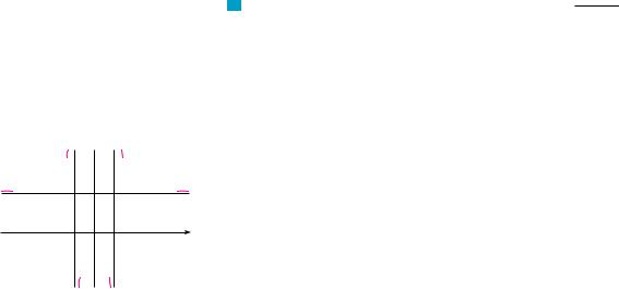
56.Coulomb’s Law states that the force of attraction between two charged particles is directly proportional to the product of the charges and inversely proportional to the square of the distance between them. The figure shows particles with charge 1 located at positions 0 and 2 on a coordinate line and a particle with charge 1 at a position x between them. It follows from Coulomb’s Law that the net force acting on the middle particle is
F x |
k |
|
k |
|
|
|
|
|
0 |
x 2 |
|
x2 |
x 2 2 |
||||
where k is a positive constant. Sketch the graph of the net force function. What does the graph say about the force?
+1 |
_1 |
+1 |
0 |
x |
x |
2 |

SECTION 4.6 GRAPHING WITH CALCULUS AND CALCULATORS |||| 315
57–60 Find an equation of the slant asymptote. Do not sketch the curve.
57. y ! |
x2 % 1 |
|
58. |
y ! |
2x3 % x2 % x % 3 |
|
|
x % 1 |
x2 % 2x |
||||||
59. y ! |
4x3 ! 2x2 % 5 |
60. |
y ! |
5x4 % x2 % x |
|
||
2x2 % x ! 3 |
x3 ! x2 % 2 |
||||||
|
|
|
|
|
|
|
|
61–66 Use the guidelines of this section to sketch the curve. In guideline D find an equation of the slant asymptote.
61. |
y ! |
!2x2 % 5x ! 1 |
62. |
y ! |
x2 % 12 |
|
|||
|
2x ! 1 |
x ! 2 |
|||||||
63. |
xy ! x2 % 4 |
64. |
y ! ex ! x |
||||||
65. |
y ! |
2x3 |
% x2 % 1 |
|
66. |
y ! |
!x % 1"3 |
|
|
|
x2 % 1 |
!x ! 1"2 |
|
||||||
|
|
|
|
|
|
|
|
|
|
67.Show that the curve y ! x ! tan!1x has two slant asymptotes: y ! x % (#2 and y ! x ! (#2. Use this fact to help sketch
the curve.
68.Show that the curve y ! sx2 % 4x has two slant asymptotes: y ! x % 2 and y ! !x ! 2. Use this fact to help sketch the curve.
69.Show that the lines y ! !b#a"x and y ! !!b#a"x are slant asymptotes of the hyperbola !x2#a2 " ! ! y2#b2 " ! 1.
70.Let f !x" ! !x3 % 1"#x. Show that
lim ' f !x" ! x2 ( ! 0
x l+"
This shows that the graph of f approaches the graph of y ! x2, and we say that the curve y ! f !x" is asymptotic to the parabola y ! x2. Use this fact to help sketch the graph of f.
71.Discuss the asymptotic behavior of f !x" ! !x4 % 1"#x in the same manner as in Exercise 70. Then use your results to help sketch the graph of f .
72.Use the asymptotic behavior of f !x" ! cos x % 1#x2 to sketch its graph without going through the curve-sketching procedure of this section.
4.6
N If you have not already read Section 1.4, you should do so now. In particular, it explains how to avoid some of the pitfalls of graphing devices by choosing appropriate viewing rectangles.
|
41,000 |
|
y=Ä |
_5 |
5 |
|
_1000 |
FIGURE 1
100
y=Ä
_3 |
2 |
_50
GRAPHING WITH CALCULUS A N D CALCULATORS
The method we used to sketch curves in the preceding section was a culmination of much of our study of differential calculus. The graph was the final object that we produced. In this section our point of view is completely different. Here we start with a graph produced by a graphing calculator or computer and then we refine it. We use calculus to make sure that we reveal all the important aspects of the curve. And with the use of graphing devices we can tackle curves that would be far too complicated to consider without technology. The theme is the interaction between calculus and calculators.
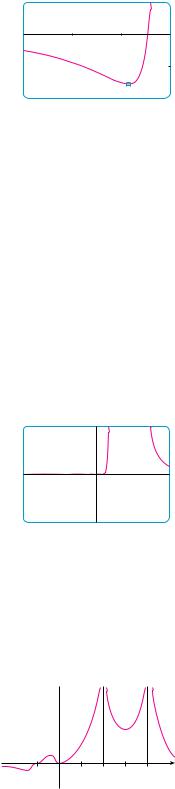
EXAMPLE 1 Graph the polynomial f !x" ! 2x6 % 3x5 % 3x3 ! 2x2. Use the graphs of f & and f # to estimate all maximum and minimum points and intervals of concavity.
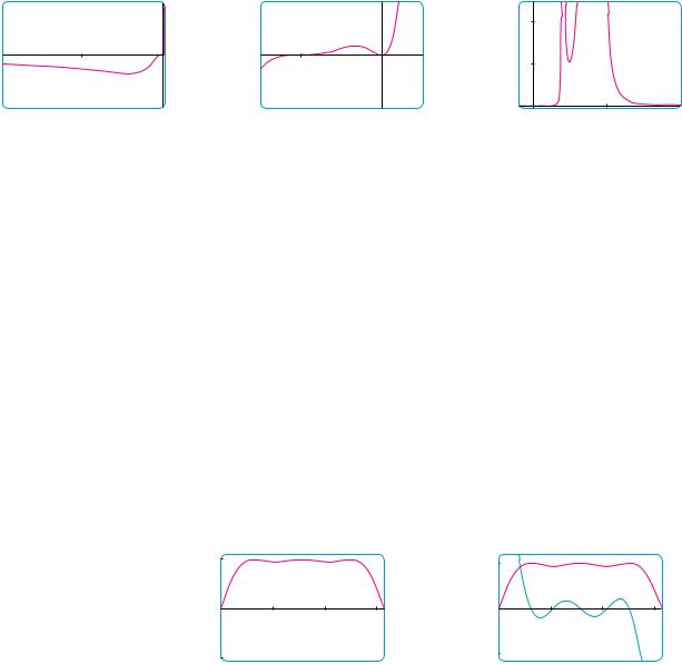
SOLUTION If we specify a domain but not a range, many graphing devices will deduce a suitable range from the values computed. Figure 1 shows the plot from one such device if we specify that !5 * x * 5. Although this viewing rectangle is useful for showing that the asymptotic behavior (or end behavior) is the same as for y ! 2x6, it is obviously hiding some finer detail. So we change to the viewing rectangle '!3, 2( by '!50, 100( shown in Figure 2.
From this graph it appears that there is an absolute minimum value of about !15.33 when x + !1.62 (by using the cursor) and f is decreasing on !!", !1.62" and increasing on !!1.62, "". Also, there appears to be a horizontal tangent at the origin and inflection points when x ! 0 and when x is somewhere between !2 and !1.
Now let’s try to confirm these impressions using calculus. We differentiate and get
f &!x" ! 12x5 % 15x4 % 9x2 ! 4x
FIGURE 2 |
f #!x" ! 60x4 % 60x3 % 18x ! 4 |

316 |||| CHAPTER 4 APPLICATIONS OF DIFFERENTIATION
20 |
|
|
When we graph f & in Figure 3 we see that f &!x" changes from negative to positive when |
|||||||||||||||||||||||||||||||
|
|
|
y=f»(x) |
|
|
|
x + !1.62; this confirms (by the First Derivative Test) the minimum value that we |
|||||||||||||||||||||||||||
|
|
|
|
|
|
found earlier. But, perhaps to our surprise, we also notice that f &!x" changes from posi- |
||||||||||||||||||||||||||||
|
|
|
|
|
|
|
|
|
||||||||||||||||||||||||||
|
|
|
|
|
|
|
|
|
tive to negative when x ! 0 and from negative to positive when x + 0.35. This means |
|||||||||||||||||||||||||
|
|
|
|
|
|
|
|
|
that f has a local maximum at 0 and a local minimum when x + 0.35, but these were |
|||||||||||||||||||||||||
_3 |
|
|
|
|
|
|
|
2 |
hidden in Figure 2. Indeed, if we now zoom in toward the origin in Figure 4, we see |
|||||||||||||||||||||||||
|
|
|
|
|
|
|
what we missed before: a local maximum value of 0 when x ! 0 and a local minimum |
|||||||||||||||||||||||||||
|
|
|
|
|
|
|
|
|
||||||||||||||||||||||||||
_5 |
|
|
value of about !0.1 when x + 0.35. |
|
|
|
|
|
|
|
|
|
|
|
|
|
|
|
|
|
|
|||||||||||||
FIGURE 3 |
|
|
What about concavity and inflection points? From Figures 2 and 4 there appear to be |
|||||||||||||||||||||||||||||||
|
inflection points when x is a little to the left of !1 and when x is a little to the right of 0. |
|||||||||||||||||||||||||||||||||
|
|
|
|
|
|
|
|
|
||||||||||||||||||||||||||
1 |
|
|
|
|
But it’s difficult to determine inflection points from the graph of f , so we graph the sec- |
|||||||||||||||||||||||||||||
|
|
|
|
|
y=Ä |
|
ond derivative f # in Figure 5. We see that f # changes from positive to negative when |
|||||||||||||||||||||||||||
|
|
|
|
|
|
x + !1.23 and from negative to positive when x + 0.19. So, correct to two decimal |
||||||||||||||||||||||||||||
_1 |
|
|
|
|
|
|
|
1 |
places, f is concave upward on !!", !1.23" and !0.19, "" and concave downward on |
|||||||||||||||||||||||||
|
|
|
|
|
|
|
!!1.23, 0.19". The inflection points are !!1.23, !10.18" and !0.19, !0.05". |
|||||||||||||||||||||||||||
|
|
|
|
|
|
|
||||||||||||||||||||||||||||
|
|
|
|
|
|
|
|
|
|
We have discovered that no single graph reveals all the important features of this |
||||||||||||||||||||||||
|
|
|
|
|
|
|
|
|
polynomial. But Figures 2 and 4, when taken together, do provide an accurate picture. M |
|||||||||||||||||||||||||
_1 |
|
|
|
|
EXAMPLE 2 Draw the graph of the function |
|
|
|
|
|
|
|
|
|
|
|
|
|
||||||||||||||||
|
V |
|
|
|
|
|
|
|
|
|
|
|
|
|
||||||||||||||||||||
|
|
|
|
|
|
|
|
|
|
|
|
|
|
|
|
|
|
|
|
|
|
|||||||||||||
FIGURE 4 |
|
|
|
|
|
|
|
f !x" ! |
x2 |
% 7x % 3 |
|
|
|
|
|
|
|
|
||||||||||||||||
10 |
|
|
|
|
|
|
|
|
|
x2 |
|
|
|
|
|
|
|
|
|
|
|
|
||||||||||||
|
|
|
|
|
|
|
|
|
|
|
|
|
|
|
|
|
|
|
|
|
|
|
|
|
|
|||||||||
_3 |
|
|
|
|
|
|
|
2 |
in a viewing rectangle that contains all the important features of the function. Estimate |
|||||||||||||||||||||||||
|
|
|
|
|
|
|
the maximum and minimum values and the intervals of concavity. Then use calculus to |
|||||||||||||||||||||||||||
|
|
|
|
|
|
|||||||||||||||||||||||||||||
|
|
|
|
|
|
|
|
|
find these quantities exactly. |
|
|
|
|
|
|
|
|
|
|
|
|
|
|
|
|
|
|
|
|
|||||
|
|
|
y=fá(x) |
|
|
|
SOLUTION Figure 6, produced by a computer with automatic scaling, is a disaster. Some |
|||||||||||||||||||||||||||
|
|
|
|
|
|
|
|
|
graphing calculators use '!10, 10( by '!10, 10( as the default viewing rectangle, so let’s |
|||||||||||||||||||||||||
|
|
|
|
|
|
|
|
|
try it. We get the graph shown in Figure 7; it’s a major improvement. |
|||||||||||||||||||||||||
_30 |
|
|
||||||||||||||||||||||||||||||||
|
|
|
The y-axis appears to be a vertical asymptote and indeed it is because |
|||||||||||||||||||||||||||||||
|
|
|
|
|
|
|
|
|
|
|||||||||||||||||||||||||
FIGURE 5 |
|
|
|
|
|
|
|
|
|
x2 |
% 7x % 3 |
|
|
|
|
|
|
|
|
|
|
|
|
|||||||||||
|
|
|
|
|
|
|
|
|
|
|
|
|
|
|
lim |
|
! " |
|
|
|
|
|
|
|
|
|||||||||
|
|
|
|
|
|
|
|
|
|
|
|
|
|
|
|
|
|
|
x2 |
|
|
|
|
|
|
|
|
|
|
|||||
|
|
|
|
|
|
|
|
|
|
|
|
|
|
|
x l0 |
|
|
|
|
|
|
|
|
|
|
|
|
|
|
|
|
|
||
|
|
|
|
|
|
|
|
|
Figure 7 also allows us to estimate the x-intercepts: about !0.5 and !6.5. The exact val- |
|||||||||||||||||||||||||
|
|
|
|
|
|
|
|
|
ues are obtained by using the quadratic formula to solve the equation x2 % 7x % 3 ! 0; |
|||||||||||||||||||||||||
|
|
|
|
|
|
|
|
|
we get x ! (!7 + s37 )#2. |
|
|
|
|
|
|
|
|
|
|
|
|
|
|
|
|
|
|
|
|
|||||
3 - 10!* |
|
|
10 |
|
|
|
|
|
|
|
|
|
|
|
|
|
|
|
|
|
|
10 |
|
|||||||||||
|
|
|
|
|
|
|
|
|
|
|
|
|
|
|
y=Ä |
|
|
|
|
|
|
|
|
|
|
|
|
|
|
|
|
y=Ä |
||
_5 |
|
|
y=Ä |
|
|
|
5 |
_10 |
|
|
|
|
|
|
10 |
|
|
|
|
_20 |
|
|
|
y=1 |
|
|
|
20 |
||||||
|
|
|
|
|
|
|
|
|
|
|
|
|
|
|
|
|
|
|
|
|
||||||||||||||
|
|
|
|
|
|
|
|
|
|
|
|
|
|
|
|
|
|
|
|
|
|
|
|
|
|
|
|
|
|
|||||
|
|
|
|
|
|
|
|
|
|
|
|
|
|
|
|
|
|
|
|
|
|
|
|
|
|
_ |
|
5 |
||||||
|
|
|
|
|
|
|
|
|
|
|
|
|
|
|
|
|
|
|
|
|
|
|
|
|
|
|
|
|
|
|
||||
|
|
|
|
|
|
|
|
|
|
|
|
|
|
|
|
|
|
|
|
|
|
|
|
|
|
|
|
|
||||||
|
|
|
|
|
|
|
|
|
_10 |
|
|
|
|
|
|
|
|
|
|
|
|
|
|
|
|
|
|
|
||||||
FIGURE 6 |
|
|
FIGURE 7 |
|
|
|
|
|
|
|
|
|
FIGURE 8 |
|
|
|
|
|||||||||||||||||
|
|
|
|
|
|
|
|
|
|
To get a better look at horizontal asymptotes, we change to the viewing rectangle |
||||||||||||||||||||||||
|
|
|
|
|
|
|
|
|
'!20, 20( by '!5, 10( in Figure 8. It appears that y ! 1 is the horizontal asymptote and |
|||||||||||||||||||||||||
|
|
|
|
|
|
|
|
|
this is easily confirmed: |
|
|
|
|
|
|
|
|
|
|
|
|
|
|
|
|
|
|
|
|
|
||||
|
|
|
|
|
|
|
|
|
|
|
lim |
|
x2 |
% 7x % 3 |
! lim |
1 % |
7 |
|
% |
|
3 |
|
! 1 |
|
|
|
||||||||
|
|
|
|
|
|
|
|
|
|
|
|
|
x2 |
|
x |
|
x2 * |
|
|
|
||||||||||||||
|
|
|
|
|
|
|
|
|
|
|
x l+" |
|
|
|
|
x l+" ) |
|
|
|
|
|
|
|
|
||||||||||
2
_3 |
0 |
y=Ä
_4
FIGURE 9
|
10 |
_10 |
y=Ä |
10 |
_10
FIGURE 10
y
_1 |
1 2 3 4 |
x |
|
FIGURE 11
SECTION 4.6 GRAPHING WITH CALCULUS AND CALCULATORS |||| 317
To estimate the minimum value we zoom in to the viewing rectangle '!3, 0( by '!4, 2( in Figure 9. The cursor indicates that the absolute minimum value is about !3.1 when x + !0.9, and we see that the function decreases on !!", !0.9" and !0, "" and increases on !!0.9, 0". The exact values are obtained by differentiating:
7 |
6 |
|
7x % 6 |
||
f &!x" ! ! |
|
! |
|
! ! |
|
x2 |
x3 |
x3 |
|||
This shows that f &!x" $ 0 when !67 ' x ' 0 and f &!x" ' 0 when x ' !67 and when
x $ 0. The exact minimum value is f (!67 ) ! !3712 + !3.08.
Figure 9 also shows that an inflection point occurs somewhere between x ! !1 and x ! !2. We could estimate it much more accurately using the graph of the second derivative, but in this case it’s just as easy to find exact values. Since
|
f #!x" ! 14 % |
18 ! |
2(7x % 9" |
|
|
x3 |
x4 |
x4 |
|
we see that f #!x" $ 0 when x $ !79 !x " 0". So f |
is concave upward on (!79 , 0) and |
|||
!0, "" and concave downward on (!", !79 ). The inflection point is (!79 , !2771 ). |
||||
|
The analysis using the first two derivatives shows that Figures 7 and 8 display all the |
|||
major aspects of the curve. |
|
|
M |
|
|
EXAMPLE 3 Graph the function f !x" ! |
x2!x % 1"3 |
||
V |
!x ! 2"2!x ! 4"4 . |
|||
|
|
|
|
|
SOLUTION Drawing on our experience with a rational function in Example 2, let’s start by graphing f in the viewing rectangle '!10, 10( by '!10, 10(. From Figure 10 we have the feeling that we are going to have to zoom in to see some finer detail and also zoom out to see the larger picture. But, as a guide to intelligent zooming, let’s first take a close look at the expression for f !x". Because of the factors !x ! 2"2 and !x ! 4"4 in the denominator, we expect x ! 2 and x ! 4 to be the vertical asymptotes. Indeed
lim |
x2!x % 1"3 |
! " and lim |
x2!x % 1"3 |
! " |
|
!x ! 2"2!x ! 4"4 |
!x ! 2"2!x ! 4"4 |
||||
x l2 |
x l4 |
|
To find the horizontal asymptotes we divide numerator and denominator by x6 :
|
|
|
|
x2 |
! |
!x % 1"3 |
1 |
)1 % |
1 |
* |
3 |
|
||||||||
x2!x % 1"3 |
|
|
|
|
|
|
|
|
|
|
x |
x |
|
|
|
|||||
|
|
x3 |
|
|
x3 |
|
|
|
||||||||||||
|
! |
|
|
|
|
|
|
|
! |
|
|
|
|
|
|
|
|
|
||
!x ! 2"2!x ! 4"4 |
|
! x ! 2"2 |
! |
!x ! 4"4 |
|
|
2 2 |
|
|
4 4 |
||||||||||
|
|
|
|
|
|
|
|
|
|
|
|
|
|
|
|
|
|
|
|
|
|
|
|
|
x2 |
|
|
x4 |
)1 ! x * )1 ! x * |
||||||||||||
|
|
|
|
|
|
|
||||||||||||||
This shows that f !x" l0 as x l+", so the x-axis is a horizontal asymptote.
It is also very useful to consider the behavior of the graph near the x-intercepts using an analysis like that in Example 11 in Section 2.6. Since x2 is positive, f !x" does not change sign at 0 and so its graph doesn’t cross the x-axis at 0. But, because of the factor !x % 1"3, the graph does cross the x-axis at !1 and has a horizontal tangent there. Putting all this information together, but without using derivatives, we see that the curve has to look something like the one in Figure 11.
318 |||| CHAPTER 4 APPLICATIONS OF DIFFERENTIATION
Now that we know what to look for, we zoom in (several times) to produce the graphs in Figures 12 and 13 and zoom out (several times) to get Figure 14.
|
0.05 |
|
0.0001 |
500 |
|
|
|
|
y=Ä |
|
y=Ä |
|
|
|
|
|
|
_100 |
1 |
_1.5 |
|
0.5 |
|
|
y=Ä |
|
|
|
|
|
_0.05 |
|
_0.0001 |
_1 _10 |
10 |
FIGURE 12 |
|
FIGURE 13 |
|
FIGURE 14 |
|
N The family of functions
f !x" ! sin!x % sin cx"
where c is a constant, occurs in applications to frequency modulation (FM) synthesis. A sine wave is modulated by a wave with a different frequency !sin cx". The case where c ! 2 is studied in Example 4. Exercise 25 explores another special case.
We can read from these graphs that the absolute minimum is about !0.02 and occurs when x + !20. There is also a local maximum + 0.00002 when x + !0.3 and a local minimum + 211 when x + 2.5. These graphs also show three inflection points near !35, !5, and !1 and two between !1 and 0. To estimate the inflection points closely we would need to graph f #, but to compute f # by hand is an unreasonable chore. If you have a computer algebra system, then it’s easy to do (see Exercise 15).
We have seen that, for this particular function, three graphs (Figures 12, 13, and 14) are necessary to convey all the useful information. The only way to display all these features of the function on a single graph is to draw it by hand. Despite the exaggerations and distortions, Figure 11 does manage to summarize the essential nature of the function. M
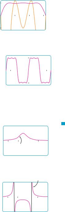
EXAMPLE 4 Graph the function f !x" ! sin!x % sin 2x". For 0 * x * (, estimate all maximum and minimum values, intervals of increase and decrease, and inflection points correct to one decimal place.
SOLUTION We first note that f is periodic with period 2(. Also, f is odd and % f !x" % * 1 for all x. So the choice of a viewing rectangle is not a problem for this function: We start
with '0, |
(( by '!1.1, 1.1(. (See Figure 15.) |
|
|
1.1 |
|
1.2 |
|
|
|
|
y=Ä |
0 |
π |
0 |
π |
|
|
|
y=f»(x) |
_1.1 |
|
_1.2 |
|
FIGURE 15 |
FIGURE 16 |
|
|
It appears that there are three local maximum values and two local minimum values in that window. To confirm this and locate them more accurately, we calculate that
f &!x" ! cos!x % sin 2x" ! !1 % 2 cos 2x"
and graph both f and f & in Figure 16.
SECTION 4.6 GRAPHING WITH CALCULUS AND CALCULATORS |||| 319
Using zoom-in and the First Derivative Test, we find the following values to one decimal place.
|
|
|
|
|
|
Intervals of increase: |
!0, 0.6", !1.0, 1.6", !2.1, 2.5" |
|
||
1.2 |
|
|
|
|
Intervals of decrease: |
!0.6, 1.0", |
!1.6, 2.1", !2.5, (" |
|
||
|
|
|
|
f |
Local maximum values: |
f !0.6" + 1, f !1.6" + 1, f !2.5" + 1 |
|
|||
|
|
|
|
Local minimum values: |
f !1.0" + 0.94, f !2.1" + 0.94 |
|
||||
0 |
|
|
|
|
π |
|
||||
|
f á |
|
|
The second derivative is |
|
|
|
|
||
|
|
|
|
|
|
|
|
|
||
_1.2 |
|
|
|
|
f #!x" ! !!1 % 2 cos 2x"2 sin!x % sin 2x" ! 4 sin 2x cos!x % sin 2x" |
|
||||
|
|
|
|
|
|
|
|
|
||
FIGURE 17 |
|
|
|
Graphing both f and f # in Figure 17, we obtain the following approximate values: |
|
|||||
|
|
|
1.2 |
|
Concave upward on: |
!0.8, 1.3", !1.8, 2.3" |
|
|||
|
|
|
|
Concave downward on: |
!0, 0.8", |
!1.3, 1.8", |
!2.3, (" |
|
||
|
|
|
|
|
|
|
||||
|
|
|
|
|
|
Inflection points: |
!0, 0", !0.8, 0.97", |
!1.3, 0.97", !1.8, 0.97", !2.3, 0.97" |
||
_2π |
|
|
|
|
2π |
|
|
|
|
|
|
|
|
|
|
|
|
|
|||
|
|
|
|
|
|
Having checked that Figure 15 does indeed represent f accurately for 0 * x * |
(, |
|||
|
|
|
|
|
|
we can state that the extended graph in Figure 18 represents f accurately for |
|
|||
|
|
|
|
|
|
!2( * x * 2(. |
|
|
|
|
|
|
|
_1.2 |
|
|
|
|
|
||
|
|
|
|
|
|
|
|
|
||
M
FIGURE 18 |
Our final example is concerned with families of functions. As discussed in Section 1.4, |
|
this means that the functions in the family are related to each other by a formula that con- |
||
|
||
|
tains one or more arbitrary constants. Each value of the constant gives rise to a member of |
|
|
the family and the idea is to see how the graph of the function changes as the constant |
|
|
changes. |
2V EXAMPLE 5 How does the graph of f !x" ! 1#!x2 % 2x % c" vary as c varies?
|
|
|
|
|
|
|
SOLUTION The graphs in Figures 19 and 20 (the special cases c ! 2 and c ! !2) show |
||||
|
|
|
|
|
|
|
two very different-looking curves. Before drawing any more graphs, let’s see what mem- |
||||
_5 |
|
|
|
|
|
4 |
bers of this family have in common. Since |
|
|||
y= |
1 |
|
|
|
|
||||||
|
|
|
|
|
|
|
1 |
|
|||
|
≈+2x+2 |
|
|
|
|
lim |
|
! 0 |
|||
|
|
|
|
|
|
|
|
|
|||
|
|
|
|
|
|
|
x l+" x2 |
% 2x % c |
|
||
|
|
_2 |
|
|
|
||||||
|
|
|
|
for any value of c, they all have the x-axis as a horizontal asymptote. A vertical asymp- |
|||||||
FIGURE 19 |
|||||||||||
tote will occur when x2 % 2x % c ! 0. Solving this quadratic equation, we get |
|||||||||||
c=2 |
|
|
|
|
|
||||||
|
|
1 |
|
x ! !1 + s1 ! c . When c $ 1, there is no vertical asymptote (as in Figure 19). When |
|||||||
|
|
|
|
y= |
≈+2x-2 |
c ! 1, the graph has a single vertical asymptote x ! !1 because |
|||||
|
|
2 |
|
|
|
|
|
|
|||
|
|
|
|
lim |
1 |
|
! lim |
1 |
|
! " |
|
|
|
|
|
|
x2 % 2x % 1 |
!x % 1"2 |
|
||||||
|
|
|
|
x l!1 |
x l!1 |
|
|
|
||||
_5 |
|
|
4 |
|
|
|
|
|
|
|
|
|
|
|
When c ' 1, there are two vertical asymptotes: x ! !1 + s1 ! c (as in Figure 20). |
||||||||||
|
|
|
|
|||||||||
|
|
|
|
Now we compute the derivative: |
|
|
|
|
|
|
||
|
|
|
|
|
f &!x" ! ! |
|
2x % 2 |
|
|
|
||
_2 |
|
|
|
|
|
|
||||||
|
|
|
!x2 % 2x % c"2 |
|
|
|
|
|||||
FIGURE 20
c=_2 |
This shows that f &!x" ! 0 when x ! !1 (if c " 1), f &!x" $ 0 when x ' !1, and |
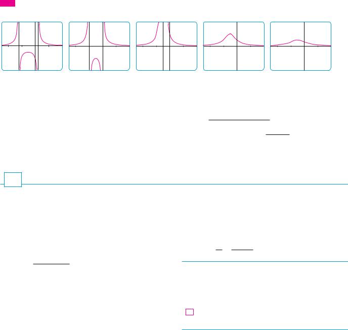
320 |||| CHAPTER 4 APPLICATIONS OF DIFFERENTIATION
TEC See an animation of Figure 21 in Visual 4.6.
f *!x" ( 0 when x % !1. For c ) 1, this means that f increases on !!', !1" and decreases on !!1, '". For c % 1, there is an absolute maximum value
f !!1" ! 1#!c ! 1". For c ( 1, f !!1" ! 1#!c ! 1" is a local maximum value and the intervals of increase and decrease are interrupted at the vertical asymptotes.
Figure 21 is a “slide show” displaying five members of the family, all graphed in the viewing rectangle $!5, 4% by $!2, 2%. As predicted, c ! 1 is the value at which a transition takes place from two vertical asymptotes to one, and then to none. As c increases from 1, we see that the maximum point becomes lower; this is explained by the fact that 1#!c ! 1" l 0 as c l '. As c decreases from 1, the vertical asymptotes become more widely separated because the distance between them is 2s1 ! c , which becomes large as c l !'. Again, the maximum point approaches the x-axis because 1#!c ! 1" l 0 as c l !'.
c=_1 |
c=0 |
c=1 |
c=2 |
c=3 |
FIGURE 21 The family of functions Ä=1/(≈+2x+c)
There is clearly no inflection point when c & 1. For c % 1 we calculate that
f #!x" ! 2!3x2 $ 6x $ 4 ! c" !x2 $ 2x $ c"3
and deduce that inflection points occur when x ! !1 " s3!c ! 1"#3. So the inflection points become more spread out as c increases and this seems plausible from the last two parts of Figure 21. M
4.6 ; EXERCISES
1–8 Produce graphs of f that reveal all the important aspects of the curve. In particular, you should use graphs of f * and f # to estimate the intervals of increase and decrease, extreme values, intervals of concavity, and inflection points.
1.f !x" ! 4x4 ! 32x3 $ 89x2 ! 95x $ 29
2.f !x" ! x6 ! 15x5 $ 75x4 ! 125x3 ! x
3.f !x" ! x6 ! 10x5 ! 400x4 $ 2500x3
x2 ! 1
4.f !x" ! 40x3 $ x $ 1
5. |
f !x" ! |
|
x |
|
x3 ! x2 ! 4x $ 1 |
|
|||
6. |
f !x" ! tan x $ 5 cos x |
|||
7. |
f !x" ! x2 ! 4x $ 7 cos x, !4 & x & 4 |
|||
8. |
f !x" ! |
ex |
||
x2 ! 9 |
|
|
||
|
|
|
|
|
9–10 Produce graphs of f that reveal all the important aspects of the curve. Estimate the intervals of increase and decrease and intervals of concavity, and use calculus to find these intervals exactly.
9. f !x" ! 1 |
1 |
8 |
1 |
|||
$ |
|
$ |
|
$ |
|
|
x |
x2 |
x3 |
||||
12 + 108
10.f !x" ! x8 ! x4
11–12
(a)Graph the function.
(b)Use l’Hospital’s Rule to explain the behavior as x l 0.
(c)Estimate the minimum value and intervals of concavity. Then use calculus to find the exact values.
11.f !x" ! x2 ln x
12.f !x" ! xe1#x

SECTION 4.6 GRAPHING WITH CALCULUS AND CALCULATORS |||| 321
13–14 Sketch the graph by hand using asymptotes and intercepts, but not derivatives. Then use your sketch as a guide to producing graphs (with a graphing device) that display the major features of the curve. Use these graphs to estimate the maximum and minimum values.
13.f !x" ! !x $ 4"!x ! 3"2
x4!x ! 1"
14.f !x" ! !2x $ 3"2!x ! 2"5
x3!x ! 5"2
CAS 15. If f is the function considered in Example 3, use a computer algebra system to calculate f * and then graph it to confirm that all the maximum and minimum values are as given in the example. Calculate f # and use it to estimate the intervals of concavity and inflection points.
CAS 16. If f is the function of Exercise 14, find f * and f # and use their graphs to estimate the intervals of increase and decrease and concavity of f.
CAS 17–22 Use a computer algebra system to graph f and to find f * and f #. Use graphs of these derivatives to estimate the intervals of increase and decrease, extreme values, intervals of concavity, and inflection points of f.
|
|
|
s |
|
|
|
|
|
|
x2# 3 |
|
|||
17. |
f !x" ! |
|
x |
18. |
f !x" ! |
|
||||||||
x2 $ x $ 1 |
|
1 |
$ x $ x4 |
|||||||||||
19. |
f !x" ! s |
|
|
|
|
, |
x & 20 |
|
|
|
|
|
||
x $ 5 sin x |
|
|
|
|
|
|||||||||
20. |
f !x" ! !x2 ! 1" earctan x |
|
|
|
|
|
|
|||||||
|
1 |
! e1# x |
|
|
|
1 |
|
|
||||||
21. |
f !x" ! |
|
|
|
|
|
|
|
22. |
f !x" ! |
|
|
|
|
1 |
$ e1# x |
1 |
$ etan x |
|||||||||||
CAS 23–24
(a)Graph the function.
(b)Explain the shape of the graph by computing the limit as x l 0$ or as x l '.
(c)Estimate the maximum and minimum values and then use calculus to find the exact values.
(d)Use a graph of f # to estimate the x-coordinates of the inflection points.
|
|
f !x" ! x1#x |
24. f !x" ! !sin x"sin x |
|
23. |
||
|
|
|
|
25.In Example 4 we considered a member of the family of functions f !x" ! sin!x $ sin cx" that occur in FM synthesis. Here we investigate the function with c ! 3. Start by graphing f in the viewing rectangle $0, ,% by $!1.2, 1.2%. How many local maximum points do you see? The graph has more than are visible to the naked eye. To discover the hidden maximum
and minimum points you will need to examine the graph of
f * very carefully. In fact, it helps to look at the graph of f # at
the same time. Find all the maximum and minimum values and inflection points. Then graph f in the viewing rectangle $!2,, 2,% by $!1.2, 1.2% and comment on symmetry.
26–33 Describe how the graph of f varies as c varies. Graph several members of the family to illustrate the trends that you discover. In particular, you should investigate how maximum and minimum points and inflection points move when c changes. You should also identify any transitional values of c at which the basic shape of the curve changes.
26. f !x" ! x3 $ cx
28. f !x" ! xsc2 ! x2
30. f !x" ! ln!x2 $ c"
1
32. f !x" ! !1 ! x2 "2 $ cx2
27. f !x" ! x4 $ cx2
29. f !x" ! e!c#x 2
cx 31. f !x" ! 1 $ c2x2
33. f !x" ! cx $ sin x
34.The family of functions f !t" ! C!e!at ! e!bt ", where a, b, and C are positive numbers and b % a, has been used to model the concentration of a drug injected into the bloodstream at time t ! 0. Graph several members of this family. What do they have in common? For fixed values of C and a, discover graphically what happens as b increases. Then use calculus to prove what you have discovered.
35.Investigate the family of curves given by f !x" ! xe!cx, where c is a real number. Start by computing the limits as x l "'. Identify any transitional values of c where the basic shape changes. What happens to the maximum or minimum points and inflection points as c changes? Illustrate by graphing several members of the family.
36.Investigate the family of curves given by the equation
f !x" ! x4 $ cx2 $ x. Start by determining the transitional value of c at which the number of inflection points changes. Then graph several members of the family to see what shapes are possible. There is another transitional value of c at which the number of critical numbers changes. Try to discover it graphically. Then prove what you have discovered.
37.(a) Investigate the family of polynomials given by the equation f !x" ! cx4 ! 2x2 $ 1. For what values of c does the curve have minimum points?
(b)Show that the minimum and maximum points of every curve in the family lie on the parabola y ! 1 ! x2. Illustrate by graphing this parabola and several members of the family.
38.(a) Investigate the family of polynomials given by the equation f !x" ! 2x3 $ cx2 $ 2x. For what values of c does the curve have maximum and minimum points?
(b)Show that the minimum and maximum points of every curve in the family lie on the curve y ! x ! x3. Illustrate by graphing this curve and several members of the family.