as a function of body length L (measured in centimeters) is W ! 0.12L2.53. If, over 10 million years, the average length of

a certain species of fish evolved from 15 cm to 20 cm at a constant rate, how fast was this species’ brain growing when the average length was 18 cm?

35.Two sides of a triangle have lengths 12 m and 15 m. The angle between them is increasing at a rate of 2&!min. How fast is the length of the third side increasing when the angle between the sides of fixed length is 60&?

36.Two carts, A and B, are connected by a rope 39 ft long that passes over a pulley P (see the figure). The point Q is on the floor 12 ft directly beneath P and between the carts. Cart A is being pulled away from Q at a speed of 2 ft!s. How fast is cart B moving toward Q at the instant when cart A is 5 ft from Q?

P

12 f t

A B

Q

37.A television camera is positioned 4000 ft from the base of a rocket launching pad. The angle of elevation of the camera has to change at the correct rate in order to keep the rocket in sight. Also, the mechanism for focusing the camera has to take into account the increasing distance from the camera to the rising rocket. Let’s assume the rocket rises vertically and its speed is 600 ft!s when it has risen 3000 ft.

(a)How fast is the distance from the television camera to the rocket changing at that moment?

(b)If the television camera is always kept aimed at the rocket, how fast is the camera’s angle of elevation changing at that same moment?

38.A lighthouse is located on a small island 3 km away from the nearest point P on a straight shoreline and its light makes four revolutions per minute. How fast is the beam of light moving along the shoreline when it is 1 km from P?

39.A plane flies horizontally at an altitude of 5 km and passes directly over a tracking telescope on the ground. When the angle of elevation is #!3, this angle is decreasing at a rate of

#!6 rad!min. How fast is the plane traveling at that time?

40.A Ferris wheel with a radius of 10 m is rotating at a rate of one revolution every 2 minutes. How fast is a rider rising when his seat is 16 m above ground level?

41.A plane flying with a constant speed of 300 km!h passes over a ground radar station at an altitude of 1 km and climbs at an angle of 30&. At what rate is the distance from the plane to the radar station increasing a minute later?

42.Two people start from the same point. One walks east at

3 mi!h and the other walks northeast at 2 mi!h. How fast is the distance between the people changing after 15 minutes?

43.A runner sprints around a circular track of radius 100 m at a constant speed of 7 m!s. The runner’s friend is standing at a distance 200 m from the center of the track. How fast is the distance between the friends changing when the distance between them is 200 m?

44.The minute hand on a watch is 8 mm long and the hour hand is 4 mm long. How fast is the distance between the tips of the hands changing at one o’clock?

3.10

y

y=Ä

{a,!f(a)} y=L(x)

FIGURE 1

LINEAR APPROXIMATIONS AND DIFFERENTIALS

We have seen that a curve lies very close to its tangent line near the point of tangency. In fact, by zooming in toward a point on the graph of a differentiable function, we noticed that the graph looks more and more like its tangent line. (See Figure 2 in Section 2.7.) This observation is the basis for a method of finding approximate values of functions.

The idea is that it might be easy to calculate a value f "a# of a function, but difficult (or even impossible) to compute nearby values of f. So we settle for the easily computed values of the linear function L whose graph is the tangent line of f at "a, f "a##. (See Figure 1.)

In other words, we use the tangent line at "a, f "a## as an approximation to the curve y ! f "x# when x is near a. An equation of this tangent line is

y ! f "a# " f '"a#"x ! a#

and the approximation

is called the linear approximation or tangent line approximation of f at a. The linear

y

y= 74+ 4x

(1,!2) y=!!!!Пггггx+3

FIGURE 2

V EXAMPLE 1 Find the linearization of the function f "x# ! sx " 3 at a ! 1 and use it to approximate the numbers s3.98 and s4.05 . Are these approximations overestimates or underestimates?

SOLUTION The derivative of f "x# ! "x " 3#1!2 is

and so we have f "1# ! 2 and f '"1# ! 14 . Putting these values into Equation 2, we see that the linearization is

The linear approximation is illustrated in Figure 2. We see that, indeed, the tangent line approximation is a good approximation to the given function when x is near l. We also see that our approximations are overestimates because the tangent line lies above the curve.

In the following table we compare the estimates from the linear approximation in Example 1 with the true values. Notice from this table, and also from Figure 2, that the tangent line approximation gives good estimates when x is close to 1 but the accuracy of the approximation deteriorates when x is farther away from 1.

_1

FIGURE 3

3

Q

y=Ïx+3+0ãããã.1

Py=Ïx+3ãããã-0.1

FIGURE 4

SECTION 3.10 LINEAR APPROXIMATIONS AND DIFFERENTIALS |||| 249

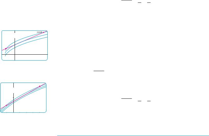
How good is the approximation that we obtained in Example 1? The next example shows that by using a graphing calculator or computer we can determine an interval throughout which a linear approximation provides a specified accuracy.

EXAMPLE 2 For what values of x is the linear approximation

sx " 3 $ 74 " 4x

accurate to within 0.5? What about accuracy to within 0.1?

This says that the linear approximation should lie between the curves obtained by shifting the curve y ! sx " 3 upward and downward by an amount 0.5. Figure 3 shows the tangent line y ! "7 " x#!4 intersecting the upper curve y ! sx " 3 " 0.5 at P and Q. Zooming in and using the cursor, we estimate that the x-coordinate of P is about !2.66 and the x-coordinate of Q is about 8.66. Thus we see from the graph that the approximation

sx " 3 $ 74 " 4x

is accurate to within 0.5 when !2.6 ( x ( 8.6. (We have rounded to be safe.) Similarly, from Figure 4 we see that the approximation is accurate to within 0.1 when

!1.1 ( x ( 3.9. M

APPLICATIONS TO PHYSICS

Linear approximations are often used in physics. In analyzing the consequences of an equation, a physicist sometimes needs to simplify a function by replacing it with its linear approximation. For instance, in deriving a formula for the period of a pendulum, physics textbooks obtain the expression aT ! !t sin $ for tangential acceleration and then replace sin $ by $ with the remark that sin $ is very close to $ if $ is not too large. [See, for example, Physics: Calculus, 2d ed., by Eugene Hecht (Pacific Grove, CA: Brooks/Cole, 2000), p. 431.] You can verify that the linearization of the function f "x# ! sin x at a ! 0 is L"x# ! x and so the linear approximation at 0 is

sin x $ x

(see Exercise 42). So, in effect, the derivation of the formula for the period of a pendulum uses the tangent line approximation for the sine function.

Another example occurs in the theory of optics, where light rays that arrive at shallow angles relative to the optical axis are called paraxial rays. In paraxial (or Gaussian) optics, both sin $ and cos $ are replaced by their linearizations. In other words, the linear approx-

N If dx " 0, we can divide both sides of Equation 3 by dx to obtain

dydx ! f '"x#

We have seen similar equations before, but now the left side can genuinely be interpreted as a ratio of differentials.

FIGURE 5

N Figure 6 shows the function in Example 3 and a comparison of dy and )y when a ! 2. The viewing rectangle is '1.8, 2.5( by '6, 18(.

y=þ+≈-2x+1

dy ëy

(2,!9)

FIGURE 6

mations became the basic theoretical tool used to design lenses. [See Optics, 4th ed., by Eugene Hecht (San Francisco: Addison-Wesley, 2002), p. 154.]

In Section 11.11 we will present several other applications of the idea of linear approximations to physics.

DIFFERENTIALS

The ideas behind linear approximations are sometimes formulated in the terminology and notation of differentials. If y ! f "x#, where f is a differentiable function, then the differential dx is an independent variable; that is, dx can be given the value of any real number. The differential dy is then defined in terms of dx by the equation

So dy is a dependent variable; it depends on the values of x and dx. If dx is given a specific value and x is taken to be some specific number in the domain of f, then the numerical value of dy is determined.

The geometric meaning of differentials is shown in Figure 5. Let P"x, f "x## and Q"x " )x, f "x " )x## be points on the graph of f and let dx ! )x. The corresponding change in y is

)y ! f "x " )x# ! f "x#

The slope of the tangent line PR is the derivative f '"x#. Thus the directed distance from S to R is f '"x# dx ! dy. Therefore dy represents the amount that the tangent line rises or falls (the change in the linearization), whereas )y represents the amount that the curve y ! f "x# rises or falls when x changes by an amount dx.

EXAMPLE 3 Compare the values of )y and dy if y ! f "x# ! x3 " x2 ! 2x " 1 and x changes (a) from 2 to 2.05 and (b) from 2 to 2.01.

SOLUTION

(a) We have

f "2# ! 23 " 22 ! 2"2# " 1 ! 9

f "2.05# ! "2.05#3 " "2.05#2 ! 2"2.05# " 1 ! 9.717625

)y ! f "2.05# ! f "2# ! 0.717625

In general, dy ! f '"x# dx ! "3x2 " 2x ! 2# dx

When x ! 2 and dx ! )x ! 0.05, this becomes

dy ! '3"2#2 " 2"2# ! 2(0.05 ! 0.7

(b)f "2.01# ! "2.01#3 " "2.01#2 ! 2"2.01# " 1 ! 9.140701

)y ! f "2.01# ! f "2# ! 0.140701

When dx ! )x ! 0.01,

SOLUTION If the radius of the sphere is measured value of r is denoted by dr lated value of V is )V, which can be

r, then its volume is V ! 43 #r3. If the error in the ! )r, then the corresponding error in the calcuapproximated by the differential

)V

V

$ dVV ! 4

3.10EXERCISES

;5. Find the linear approximation of the function f !x" ! s1 % x at a ! 0 and use it to approximate the numbers s0.9 and s0.99 . Illustrate by graphing f and the tangent line.

;6. Find the linear approximation of the function t!x" ! s3 1 $ x at a ! 0 and use it to approximate the numbers s3 0.95 and s3 1.1 . Illustrate by graphing t and the tangent line.

;7–10 Verify the given linear approximation at a ! 0. Then determine the values of x for which the linear approximation is accurate to within 0.1.

11–14 Find the differential of each function.

15–18 (a) Find the differential dy and (b) evaluate dy for the given values of x and dx.

19–22 Compute #y and dy for the given values of x and

dx ! #x. Then sketch a diagram like Figure 5 showing the line segments with lengths dx, dy, and #y.

19.y ! 2x % x2, x ! 2, #x ! %0.4

20.y ! sx , x ! 1, #x ! 1

21.y ! 2$x, x ! 4, #x ! 1

22.y ! ex, x ! 0, #x ! 0.5

23–28 Use a linear approximation (or differentials) to estimate the given number.

29–31 Explain, in terms of linear approximations or differentials, why the approximation is reasonable.

(a)Find the linearizations of f , t, and h at a ! 0. What do you notice? How do you explain what happened?

;(b) Graph f , t, and h and their linear approximations. For which function is the linear approximation best? For which is it worst? Explain.

33.The edge of a cube was found to be 30 cm with a possible error in measurement of 0.1 cm. Use differentials to estimate the maximum possible error, relative error, and percentage error in computing (a) the volume of the cube and (b) the surface area of the cube.

34.The radius of a circular disk is given as 24 cm with a maximum error in measurement of 0.2 cm.

(a)Use differentials to estimate the maximum error in the calculated area of the disk.

(b)What is the relative error? What is the percentage error?

35.The circumference of a sphere was measured to be 84 cm with a possible error of 0.5 cm.

(a)Use differentials to estimate the maximum error in the calculated surface area. What is the relative error?

(b)Use differentials to estimate the maximum error in the calculated volume. What is the relative error?

36.Use differentials to estimate the amount of paint needed to apply a coat of paint 0.05 cm thick to a hemispherical dome with diameter 50 m.

37.(a) Use differentials to find a formula for the approximate volume of a thin cylindrical shell with height h, inner radius r, and thickness #r.

(b)What is the error involved in using the formula from part (a)?

38.One side of a right triangle is known to be 20 cm long and the opposite angle is measured as 30", with a possible error of !1".

(a)Use differentials to estimate the error in computing the length of the hypotenuse.

(b)What is the percentage error?

39.If a current I passes through a resistor with resistance R, Ohm’s Law states that the voltage drop is V ! RI. If V is constant and R is measured with a certain error, use differentials to show that the relative error in calculating I is approximately the same (in magnitude) as the relative error in R.

40.When blood flows along a blood vessel, the flux F (the volume of blood per unit time that flows past a given point) is proportional to the fourth power of the radius R of the blood vessel:

F ! kR4

(This is known as Poiseuille’s Law; we will show why it is true in Section 8.4.) A partially clogged artery can be expanded by an operation called angioplasty, in which a balloon-tipped catheter is inflated inside the artery in order to widen it and restore the normal blood flow.

Show that the relative change in F is about four times the relative change in R. How will a 5% increase in the radius affect the flow of blood?

41.Establish the following rules for working with differentials (where c denotes a constant and u and v are functions of x).

42.On page 431 of Physics: Calculus, 2d ed., by Eugene Hecht

(Pacific Grove, CA: Brooks/Cole, 2000), in the course of deriving the formula T ! 2&sL$t for the period of a pendulum of length L, the author obtains the equation

than 2% out to about 20°.”

(a) Verify the linear approximation at 0 for the sine function:

sin x # x

;(b) Use a graphing device to determine the values of x for which sin x and x differ by less than 2%. Then verify Hecht’s statement by converting from radians to degrees.

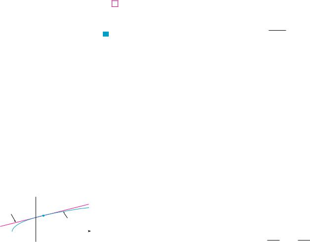
43.Suppose that the only information we have about a function f is that f !1" ! 5 and the graph of its derivative is as shown.

(a)Use a linear approximation to estimate f !0.9" and f !1.1".

(b)Are your estimates in part (a) too large or too small? Explain.

y

44.Suppose that we don’t have a formula for t!x" but we know that t!2" ! %4 and t'!x" ! sx2 $ 5 for all x.

(a)Use a linear approximation to estimate t!1.95" and t!2.05".

(b)Are your estimates in part (a) too large or too small? Explain.