Добавил:

PavelEngineer Опубликованный материал нарушает ваши авторские права? Сообщите нам.

Вуз:

Севастопольский Государственный Университет

Предмет:

[НЕСОРТИРОВАННОЕ]

Файл:

[James_Stewart]_Single_Variable_Calculus_Early_Tr(BookFi).pdf

Скачиваний:

Добавлен:

30.12.2019

Размер:

18.09 Mб

Скачать

☆

<<< < Предыдущая 6 7 8 9 10 11 12 13 14 15 16 1718 / 9118 19 20 21 22 23 24 25 26 27 28 29 30 > Следующая >>>

					SECTION 3.2 THE PRODUCT AND QUOTIENT RULES \|\|\|\| 183

		f		segments L1 and L2 to be tangent to the parabola at the transition points P and Q. (See the ﬁg-
LÁ	P	f		ure.) To simplify the equations you decide to place the origin at P.
LÁ	P
				1. (a)	Suppose the horizontal distance between P and Q is 100 ft. Write equations in a, b, and c
		Q			that will ensure that the track is smooth at the transition points.
		Lª ;		(b)	Solve the equations in part (a) for a, b, and c to ﬁnd a formula for f ! x".
		Lª ;		(c)	Plot L1, f, and L2 to verify graphically that the transitions are smooth.
				(d)	Find the difference in elevation between P and Q.
				2. The solution in Problem 1 might look smooth, but it might not feel smooth because the piece-
				wise deﬁned function [consisting of L1! x" for x & 0, f ! x" for 0 # x # 100, and L2! x" for
				x $ 100] doesn’t have a continuous second derivative. So you decide to improve the design by
				using a quadratic function q! x" ! ax2 " bx " c only on the interval 10 # x # 90 and con-
				necting it to the linear functions by means of two cubic functions:
					t! x" ! kx3 " lx2 " mx " n	0 # x & 10
					h! x" ! px3 " qx2 " rx " s	90 & x # 100
				(a)	Write a system of equations in 11 unknowns that ensure that the functions and their ﬁrst
					two derivatives agree at the transition points.
			CAS	(b)	Solve the equations in part (a) with a computer algebra system to ﬁnd formulas for
					q! x", t! x", and h! x".
				(c)	Plot L1, t, q, h, and L2, and compare with the plot in Problem 1(c).

3.2 THE PRODUCT AND QUOTIENT RULES

The formulas of this section enable us to differentiate new functions formed from old functions by multiplication or division.

ë√	u!ë√	ëu!ë√
√	u√	√!ëu

	u	ëu
FIGURE 1

The geometry of the Product Rule

THE PRODUCT RULE

| By analogy with the Sum and Difference Rules, one might be tempted to guess, as Leibniz did three centuries ago, that the derivative of a product is the product of the derivatives. We can see, however, that this guess is wrong by looking at a particular example. Let f !x" ! x and t! x" ! x2. Then the Power Rule gives f %! x" ! 1 and t%! x" ! 2x. But ! ft"!x" ! x3, so ! ft"%! x" ! 3x2. Thus ! ft"% " f %t%. The correct formula was discovered by Leibniz (soon after his false start) and is called the Product Rule.

Before stating the Product Rule, let’s see how we might discover it. We start by assuming that u ! f ! x" and v ! t! x" are both positive differentiable functions. Then we can interpret the product uv as an area of a rectangle (see Figure 1). If x changes by an amount (x, then the corresponding changes in u and v are

(u ! f ! x " (x" ! f !x" (v ! t! x " (x" ! t!x"

and the new value of the product, !u " (u"!v " (v", can be interpreted as the area of the large rectangle in Figure 1 (provided that (u and (v happen to be positive).

The change in the area of the rectangle is

1(!uv" ! !u " (u"!v " (v" ! uv ! u (v " v (u " (u (v

!the sum of the three shaded areas

184 |||| CHAPTER 3 DIFFERENTIATION RULES

N Recall that in Leibniz notation the deﬁnition of a derivative can be written as

dy ! lim (y dx (x l0 (x

If we divide by (x, we get
	(!uv"	! u	(v	" v	(u
	(x	! u	(x	" v	(x

If we now let (x l 0, we get the derivative of uv:

!uv" ! lim

(!uv"

! lim

(

(x l0

! u lim

" v lim

(x l0

! u

" v

" 0 !

!uv" ! u

" v

" (u ((vx

" v ((ux " (u ((vx ) ( lim (u)( lim (v )

(x l0 (x l0 (x

NIn prime notation:

!ft"% ! ft% " tf %

N Figure 2 shows the graphs of the function f of Example 1 and its derivative f %. Notice that

f %! x" is positive when f is increasing and negative when f is decreasing.

	3
	f»
_3	1.5
	f
	_1

FIGURE 2

(Notice that (u l 0 as (x l 0 since f is differentiable and therefore continuous.) Although we started by assuming (for the geometric interpretation) that all the quanti-

ties are positive, we notice that Equation 1 is always true. (The algebra is valid whether u, v, (u, and (v are positive or negative.) So we have proved Equation 2, known as the Product Rule, for all differentiable functions u and v.

THE PRODUCT RULE If f and t are both differentiable, then

dxd & f ! x"t! x"' ! f !x" dxd & t! x"' " t! x" dxd & f ! x"'

In words, the Product Rule says that the derivative of a product of two functions is the ﬁrst function times the derivative of the second function plus the second function times the derivative of the ﬁrst function.

EXAMPLE 1

(a)If f !x" ! xex, ﬁnd f %! x".

(b)Find the nth derivative, f !n"! x".

SOLUTION

(a) By the Product Rule, we have

f %!x" ! dxd !xex " ! x dxd !ex " " ex dxd ! x"

!xex " ex ) 1 ! ! x " 1"ex

(b)Using the Product Rule a second time, we get

f '! x" ! dxd &!x " 1" ex' ! ! x " 1" dxd !ex " " ex dxd ! x " 1" ! ! x " 1" ex " ex ! 1 ! ! x " 2" ex

N In Example 2, a and b are constants. It is customary in mathematics to use letters near the beginning of the alphabet to represent constants and letters near the end of the alphabet to represent variables.

SECTION 3.2 THE PRODUCT AND QUOTIENT RULES ||||

185

Further applications of the Product Rule give

f *! x" ! ! x " 3" ex

f !4"! x" ! ! x " 4" ex

In fact, each successive differentiation adds another term ex, so

f !n"! x" ! ! x " n" ex

EXAMPLE 2 Differentiate the function f !t" ! s

!a " bt".

SOLUTION 1 Using the Product Rule, we have

f %!t" ! st

(st )

!a " bt" " !a " bt"

! s

! b " !a " bt" ! 21 t!1%2

! bs

a " bt

a " 3bt

2st

SOLUTION 2 If we ﬁrst use the laws of exponents to rewrite f !t", then we can proceed directly without using the Product Rule.

f !t" ! ast " btst ! at1%2 " bt3%2

f %!t" ! 12 at!1%2 " 32 bt1%2

which is equivalent to the answer given in Solution 1.

Example 2 shows that it is sometimes easier to simplify a product of functions than to use the Product Rule. In Example 1, however, the Product Rule is the only possible method.

EXAMPLE 3 If f ! x" ! sx t!x", where t!4" ! 2 and t%!4" ! 3, ﬁnd f %!4".

SOLUTION Applying the Product Rule, we get

f %!x" !

t! x"] ! s

& t! x"' " t! x"

]

!1%2

t! x"

! sx t%!x" " t!x"

! sx t%! x" "

) 2 x

t!4"

f %!4" ! s4 t%!4" "

2 ) 3

! 6.5

2 ) 2

THE QUOTIENT RULE

We ﬁnd a rule for differentiating the quotient of two differentiable functions u ! f !x" and v ! t! x" in much the same way that we found the Product Rule. If x, u, and v change by amounts (x, (u, and (v, then the corresponding change in the quotient u%v is

	u u " (u				u		!u " (u"v ! u!v " (v"		v(u ! u(v
((		) !		!		!		!
((	v	) !	v " (v	!	v	!	v!v " (v"	!	v!v " (v"

186 |||| CHAPTER 3 DIFFERENTIATION RULES

N In prime notation:
(t) !		t2
	f %	tf % ! ft%

N We can use a graphing device to check that the answer to Example 4 is plausible. Figure 3 shows the graphs of the function of Example 4 and its derivative. Notice that when y grows rapidly (near !2), y% is large. And when y grows slowly, y% is near 0.

1.5

y»

_1.5

FIGURE 3

! u

d u

! lim

(!u%v"

! lim

dx ( v )

v!v " (v"

(x l0

As (x l0, (v l0 also, because v ! t! x" is differentiable and therefore continuous. Thus, using the Limit Laws, we get

v lim

! u lim

! u

d u

(x l0

(

) !

v lim !v " (v"

(x l0

THE QUOTIENT RULE If f and t are differentiable, then

+ !

t! x"

& f !x"' ! f ! x"

&t! x"'

f ! x"

t! x"

& t! x"' 2

In words, the Quotient Rule says that the derivative of a quotient is the denominator times the derivative of the numerator minus the numerator times the derivative of the denominator, all divided by the square of the denominator.

The Quotient Rule and the other differentiation formulas enable us to compute the derivative of any rational function, as the next example illustrates.

	EXAMPLE 4 Let y !		x2	" x ! 2				. Then
V		!x3 " 6"			d	! x2	" x ! 2" ! ! x2 " x ! 2"		d	! x3 " 6"
					d				d
									dx
	y% !				dx				dx
	y% !							! x3 " 6"2
								! x3 " 6"2

!!x3 " 6"!2x " 1" ! ! x2 " x ! 2"!3x2 " ! x3 " 6"2

!!2x4 " x3 " 12x " 6" ! !3x4 " 3x3 ! 6x2 " ! x3 " 6"2

!	!x4	! 2x3 " 6x2 " 12x " 6	M
		! x3 " 6"2

	EXAMPLE 5 Find an equation of the tangent line to the curve y ! ex%!1 " x2 " at the
V
point (1, 21 e).
SOLUTION According to the Quotient Rule, we have
			!1 " x2 "	d	!ex " ! ex			d	!1 " x2	"
	dy		!1 " x2 "		!ex " ! ex				!1 " x2	"
	dy	!		dx			dx
	dx	!			!1 " x2 "2
		!	!1 " x2 "ex ! ex!2x"			!		ex!1 ! x"2
		!	!1 " x2 "2			!		!1 " x2 "2

SECTION 3.2 THE PRODUCT AND QUOTIENT RULES |||| 187

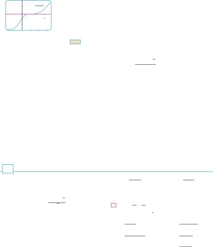
	2.5	«			So the slope of the tangent line at (1, 21 e) is
	y=	«
		1+≈			dy
					dy	! 0
		y=1	e		dx ,x!1	! 0
		y=1	e		dx ,x!1
		2
_2				3.5	This means that the tangent line at (1, 21 e) is horizontal and its equation is y ! 21 e. [See
_2	0			3.5	Figure 4. Notice that the function is increasing and crosses its tangent line at (1, 21 e).]		M

FIGURE 4

TABLE OF DIFFERENTIATION FORMULAS

N OT E Don’t use the Quotient Rule every time you see a quotient. Sometimes it’s easier to rewrite a quotient ﬁrst to put it in a form that is simpler for the purpose of differentiation. For instance, although it is possible to differentiate the function

F! x" ! 3x2 " 2sx x

using the Quotient Rule, it is much easier to perform the division ﬁrst and write the function as

F! x" ! 3x " 2x!1%2

before differentiating.

We summarize the differentiation formulas we have learned so far as follows.

d	!c" ! 0	d		! xn " ! nxn!1		d	!ex " ! ex
	!c" ! 0	dx		! xn " ! nxn!1		dx	!ex " ! ex
dx		dx				dx
!cf "% ! cf %		! f " t"% ! f % " t%				! f ! t"% ! f % ! t%
			f	%	tf % ! ft%
! ft"% ! ft% " tf %		(		) !
! ft"% ! ft% " tf %		(	t	) !	t2

3.2EXERCISES

1.Find the derivative of y ! ! x2 " 1"! x3 " 1" in two ways: by using the Product Rule and by performing the multiplication ﬁrst. Do your answers agree?

2.Find the derivative of the function

F! x" ! x ! 3xsx sx

in two ways: by using the Quotient Rule and by simplifying ﬁrst. Show that your answers are equivalent. Which method do you prefer?

3–26 Differentiate.
3.	f ! x" ! ! x3 " 2x" ex		4.	t! x" ! s			ex
						x
5.	y !	ex	6.	y !	ex
		x2			1 " x

t3x ! 1

7.! x" ! 2x " 1

9.V! x" ! !2x3 " 3"! x4 ! 2x"

10.Y!u" ! ! u!2 " u!3"! u5 ! 2u2"

11.F! y" ! (y12 ! y34 )! y " 5y3"

12.R!t" ! ! t " et"(3 ! st )

13.y ! 1 ! x2

t2 " 2

15. y ! t4 ! 3t2 " 1

17. y ! !r2 ! 2r" er

8. f !t" ! 4 " t2

x " 1

14. y ! x3 " x ! 2

16. y ! ! t ! 1"2

18. y ! s " kes

188

|||| CHAPTER 3 DIFFERENTIATION RULES

y !

v3 ! 2vs

19.

20.

z ! w3%2!w " cew"

t ! s

21.

f ! t" !

22.

t! t" !

2 " s

t1%3

23.

f ! x" !

24.

f ! x" !

1 ! xex

B " Cex

x " ex

25.

f ! x" !

26.

f ! x" !

ax " b

x "

cx " d

27–30 Find f %! x" and f '! x".

27.

f ! x" ! x4ex

28.

f ! x" ! x5%2ex

29.

f ! x" !

30.

f ! x" !

1 " 2x

3 " ex

31–32 Find an equation of the tangent line to the given curve at the speciﬁed point.

31. y !	2x		,	!1, 1"	32. y !	ex	, !1, e"
31. y !	x "	1	,	!1, 1"	32. y !	x	, !1, e"
	x "	1				x

33–34 Find equations of the tangent line and normal line to the given curve at the speciﬁed point.

		s
33. y ! 2xex, !0, 0"	34. y !	s	x	,	!4, 0.4"
33. y ! 2xex, !0, 0"	34. y !	x " 1		,	!4, 0.4"
		x " 1

35. (a) The curve y ! 1%!1 " x2" is called a witch of Maria Agnesi. Find an equation of the tangent line to this curve at the point (!1, 12 ).

;(b) Illustrate part (a) by graphing the curve and the tangent line on the same screen.

36.(a) The curve y ! x%!1 " x2 " is called a serpentine. Find an equation of the tangent line to this curve at the point !3, 0.3".

;(b) Illustrate part (a) by graphing the curve and the tangent line on the same screen.

37.(a) If f ! x" ! ex%x3, ﬁnd f %! x".

;(b) Check to see that your answer to part (a) is reasonable by comparing the graphs of f and f %.

38.(a) If f ! x" ! x%! x2 ! 1", ﬁnd f %! x".

;(b) Check to see that your answer to part (a) is reasonable by comparing the graphs of f and f %.

39.(a) If f ! x" ! ! x ! 1" ex, ﬁnd f %! x" and f '! x".

;(b) Check to see that your answers to part (a) are reasonable by comparing the graphs of f , f %, and f '.

40.	(a) If f ! x" ! x%! x2 " 1", ﬁnd f %! x" and f '! x".
;	(b) Check to see that your answers to part (a) are reasonable
	by comparing the graphs of f , f %, and f '.
41.	If f ! x" ! x2%!1 " x", ﬁnd f '!1".
42.	If t! x" ! x%ex, ﬁnd t!n"! x".
43.	Suppose that f !5" ! 1, f %!5" ! 6, t!5" ! !3, and t%!5" ! 2.
	Find the following values.		! f%t"%!5"
	(a) ! ft"%!5"	(b)	! f%t"%!5"
	(c) ! t%f "%!5"
44.	Suppose that f !2" ! !3, t!2" ! 4, f %!2" ! !2, and
	t%!2" ! 7. Find h%!2".		h! x" ! f !x" t! x"
	(a) h! x" ! 5f !x" ! 4t! x"	(b)	h! x" ! f !x" t! x"
	(c) h! x" ! f ! x"	(d)	h! x" !		t! x"
	t! x"			1 " f ! x"
45.	If f ! x" ! ext! x", where t!0" ! 2 and t%!0" ! 5, ﬁnd f %!0".
46.	If h!2" ! 4 and h%!2" ! !3, ﬁnd
	dxd (h!xx" ),x!2
47.	If f and t are the functions whose graphs are shown, let
	u! x" ! f ! x"t! x" and v! x" ! f ! x"%t! x".
	(a) Find u%!1".	(b)	Find v%!5".
	y
		f	g
	1		g
	1
	0	1		x

48.Let P! x" ! F! x"G! x" and Q! x" ! F! x"%G! x", where F and G are the functions whose graphs are shown.

(a) Find P%!2".

(b) Find Q%!7".

y
		F
1		G
0	1	x

<<< < Предыдущая 6 7 8 9 10 11 12 13 14 15 16 1718 / 9118 19 20 21 22 23 24 25 26 27 28 29 30 > Следующая >>>

Соседние файлы в предмете [НЕСОРТИРОВАННОЕ]

#
05.02.202055.36 Mб19Calculus, 7th Edition ( PDFDrive.com ).pdf
#
30.12.201945.82 Mб41Complete Solutions Manual for_ SINGLE VARIABLE CALCULUS Early Transcendentals 7th Edition by Stewart ( PDFDrive.com ).pdf
#
30.12.201918.09 Mб35[James_Stewart]_Single_Variable_Calculus_Early_Tr(BookFi).pdf