Добавил:

PavelEngineer Опубликованный материал нарушает ваши авторские права? Сообщите нам.

Вуз:

Севастопольский Государственный Университет

Предмет:

[НЕСОРТИРОВАННОЕ]

Файл:

[James_Stewart]_Single_Variable_Calculus_Early_Tr(BookFi).pdf

Скачиваний:

Добавлен:

30.12.2019

Размер:

18.09 Mб

Скачать

☆

<<< < Предыдущая 1 23 / 913 4 5 6 7 8 9 10 11 12 13 14 15 16 17 18 19 20 21 22 23 24 25 > Следующая >>>

TO THE STUDENT

Reading a calculus textbook is different from reading a newspaper or a novel, or even a physics book. Don’t be discouraged if you have to read a passage more than once in order to understand it. You should have pencil and paper and calculator at hand to sketch a diagram or make a calculation.

Some students start by trying their homework problems and read the text only if they get stuck on an exercise. I suggest that a far better plan is to read and understand a section of the text before attempting the exercises. In particular, you should look at the deﬁnitions to see the exact meanings of the terms. And before you read each example, I suggest that you cover up the solution and try solving the problem yourself. You’ll get a lot more from looking at the solution if you do so.

Part of the aim of this course is to train you to think logically. Learn to write the solutions of the exercises in a connected, step-by-step fashion with explanatory sentences— not just a string of disconnected equations or formulas.

The answers to the odd-numbered exercises appear at the back of the book, in Appendix I. Some exercises ask for a verbal explanation or interpretation or description. In such cases there is no single correct way of expressing the answer, so don’t worry that you haven’t found the deﬁnitive answer. In addition, there are often several different forms in which to express a numerical or algebraic answer, so if your answer differs from mine, don’t immediately assume you’re wrong. For example, if the answer given in the back of the book is s2 1 and you obtain 1 (1 s2), then you’re right and rationalizing the denominator will show that the answers are equivalent.

The icon ; indicates an exercise that deﬁnitely requires the use of either a graphing calculator or a computer with graphing software. (Section 1.4 discusses the use of these graphing devices and some of the pitfalls that you may encounter.) But that doesn’t mean that graphing devices can’t be used to check your work on the other exercises as well. The symbol CAS is reserved for problems in which the full resources of a computer algebra

xxii

system (like Derive, Maple, Mathematica, or the TI-89/92) are required. You will also encounter the symbol |, which warns you against committing an error. I have placed this symbol in the margin in situations where I have observed that a large proportion of my students tend to make the same mistake.

Tools for Enriching Calculus, which is a companion to this text, is referred to by means of the symbol TEC and can be accessed from www.stewartcalculus.com. It directs you to

modules in which you can explore aspects of calculus for which the computer is particularly useful. TEC also provides Homework Hints for representative exercises that are indicated by printing the exercise number in red: 15. These homework hints ask you questions that allow you to make progress toward a solution without actually giving you the answer. You need to pursue each hint in an active manner with pencil and paper to work out the details. If a particular hint doesn’t enable you to solve the problem, you can click to reveal the next hint.

An optional CD-ROM that your instructor may have asked you to purchase is the Interactive Video Skillbuilder, which contains videos of instructors explaining two or three of the examples in every section of the text. Also on the CD is a video in which I offer advice on how to succeed in your calculus course.

I recommend that you keep this book for reference purposes after you ﬁnish the course. Because you will likely forget some of the speciﬁc details of calculus, the book will serve as a useful reminder when you need to use calculus in subsequent courses. And, because this book contains more material than can be covered in any one course, it can also serve as a valuable resource for a working scientist or engineer.

Calculus is an exciting subject, justly considered to be one of the greatest achievements of the human intellect. I hope you will discover that it is not only useful but also intrinsically beautiful.

JAMES STEWART

xxiii

DIAGNOSTIC TESTS

Success in calculus depends to a large extent on knowledge of the mathematics that precedes calculus: algebra, analytic geometry, functions, and trigonometry. The following tests are intended to diagnose weaknesses that you might have in these areas. After taking each test you can check your answers against the given answers and, if necessary, refresh your skills by referring to the review materials that are provided.

ADIAGNOSTIC TEST: ALGEBRA

1.Evaluate each expression without using a calculator.

(a)	3 4	(b)	34			(c)	3 4
(d)	523	(e)		2	2	(f)	16 3 4
	521		3

2.Simplify each expression. Write your answer without negative exponents.

(a)s200 s32

(b)3a3b3 4ab2 2

3x3 2y3 2

(c)x2y 1 2

3.Expand and simplfy.

(a) 3 x 6 4 2x 5									(b) x 3 4x 5
(c) (s		s		)(s		s		)	(d) 2x 3 2
	a		b		a		b
(e) x 2 3

4.Factor each expression.

(a)4x2 25

(e)3x3 2 9x1 2 6x 1 2

5.Simplify the rational expression.

(a)	x2	3x 2
	x2 x 2

(c)		x2	x 1
	x2	4	x	2

(b) 2x2 5x 12

(d) x4 27x

(f) x3y 4xy

(b)	2x2 x 1			x 3
(b)		x2 9		2x 1
		x2 9		2x 1
	y		x
(d)	x		y
	x		y


	1		1
	y		x
	y		x

xxiv

DIAGNOSTIC TESTS |||| xxv

6. Rationalize the expression and simplify.

	s			s
(a)	s	10	(b)	s	4	h 2

	s5 2					h
	s5 2					h
7. Rewrite by completing the square.
(a)	x2 x 1		(b)	2x2		12x 11

8. Solve the equation. (Find only the real solutions.)

(a)	x 5 14 21 x	(b)	2x	2x 1
			x 1	x

(c)	x2 x 12 0	(d)	2x2 4x 1 0
(e)	x4 3x2 2 0	(f)	3 x 4 10

(g)2x 4 x 1 2 3 s4 x 0

9.Solve each inequality. Write your answer using interval notation.

(a)	4 5 3x 17	(b)	x2 2x 8
(c)	x x 1 x 2 0	(d)	x 4 3

(e)2x 3 1

10.State whether each equation is true or false.

(a) p q 2 p2 q2

(b)

(c)

a b

(d)

1 TC

1 T

a2 b2

(e)

(f)

1 x

x y

a x b x

a b

ANSWERS TO DIAGNOSTIC TEST A: ALGEBRA

(a) 81

(b)

(c)

(a) 5s2 2s10

(b)

s4 h 2

(d) 25

(e)

(f)

(a) 6

(b)

48a5b7

(c)

(a) (x 2 )

(b)

2 x 3 7

9y7

4x2 7x 15

(a) 11x 2

(b)

(a) 6

(b) 1

(c)

3, 4

(d)

4x2 12x 9

(d) 1 21 s

(e) 1, s

(f)

32 , 223

(e) x3 6x2 12x 8

(g) 5

(a) 2x 5 2x 5

(b)

2x 3 x 4

(a) 4, 3

(b)

2, 4

(d)

x x 3 x2 3x 9

(e) 3x 1 2 x 1 x 2

(f)

xy x 2 x 2

(d)

1, 7

(e) 1, 4

x 2

x 1

(a)

(b)

x 3

10.

(a) False

(b) True

(c)

False

(c)

(d)

x y

(d) False

(e) False

(f)

True

If you have had difﬁculty with these problems, you may wish to consult the Review of Algebra on the website www.stewartcalculus.com.

xxvi |||| DIAGNOSTIC TESTS

BDIAGNOSTIC TEST: ANALYTIC GEOMETRY

1.Find an equation for the line that passes through the point 2, 5 and

(a)has slope 3

(b)is parallel to the x-axis

(c)is parallel to the y-axis

(d)is parallel to the line 2x 4y 3

2.Find an equation for the circle that has center 1, 4 and passes through the point 3, 2 .

3.Find the center and radius of the circle with equation x2 y2 6x 10y 9 0.

4.Let A 7, 4 and B 5, 12 be points in the plane.

(a)Find the slope of the line that contains A and B.

(b)Find an equation of the line that passes through A and B. What are the intercepts?

(c)Find the midpoint of the segment AB.

(d)Find the length of the segment AB.

(e)Find an equation of the perpendicular bisector of AB.

(f)Find an equation of the circle for which AB is a diameter.

5.Sketch the region in the xy-plane deﬁned by the equation or inequalities.

(a)	1 y 3	(b)	x 4 and y 2
(c)	y 1 21 x	(d)	y x2 1
(e)	x2 y2 4	(f)	9x2 16y2 144

ANSWERS TO DIAGNOSTIC TEST B: ANALYTIC GEOMETRY

(a) y 3x 1

(b) y 5

5. (a)

(b)

(c)

(d) y 21 x 6

y=1-

21 x

x 1 2 y 4 2 52

4 x

Center 3, 5 , radius 5

(a) 34

(b) 4x 3y 16 0; x-intercept 4, y-intercept 163

(d)

(e)

(f )

≈+¥=4

(d) 20

(e) 3x 4y 13

1 x

2 x

(f) x 1 2 y 4 2 100

y=≈-1

If you have had difﬁculty with these problems, you may wish to consult the Review of Analytic Geometry on the website www.stewartcalculus.com.

DIAGNOSTIC TESTS |||| xxvii

C DIAGNOSTIC TEST: FUNCTIONS

y
1
0	1	x

FIGURE FOR PROBLEM 1

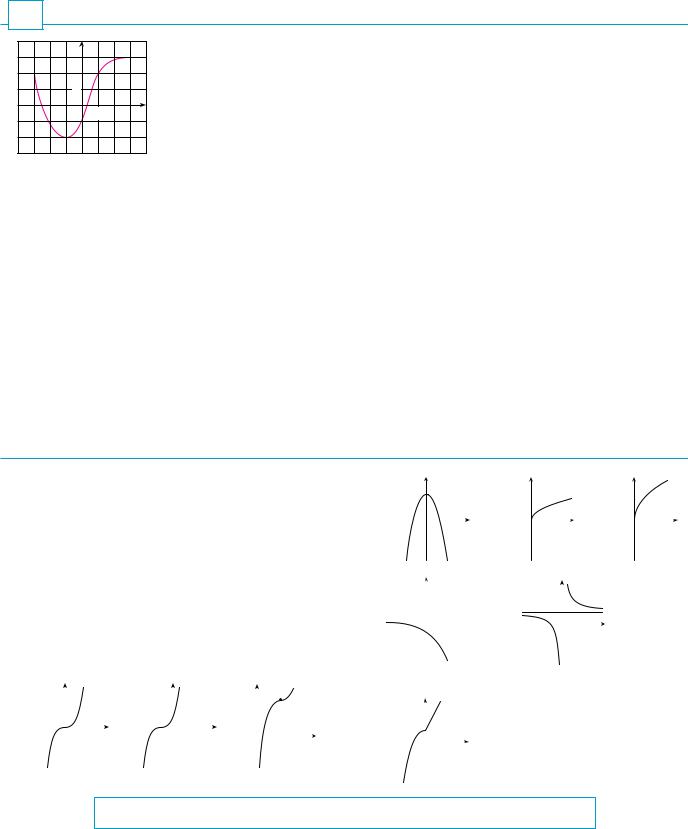
1.The graph of a function f is given at the left.

(a)State the value of f 1 .

(b)Estimate the value of f 2 .

(c)For what values of x is f x 2?

(d)Estimate the values of x such that f x 0.

(e)State the domain and range of f.

If f x x3, evaluate the difference quotient

f 2 h f 2

and simplify your answer.

Find the domain of the function.

(a)

f x

2x 1

(b)

t x

(c)

h x s

4 x

x2 1

x 2

How are graphs of the functions obtained from the graph of f ?

(a)

y f x

(b)

y 2 f x 1

(c)

y f x 3 2

Without using a calculator, make a rough sketch of the graph.

(a)

y x3

(b)

y x 1 3

(c)

y x 2 3 3

(d)

y 4 x2

(e)

y s

(f)

y 2 s

(g)

y 2x

(h) y 1 x 1

Let f x

1 x2

x 0

2x 1

x 0

(a)

Evaluate f 2 and f 1 . (b)

Sketch the graph of f.

If f x x2 2x 1 and t x 2x 3, ﬁnd each of the following functions.

(a)

f t

(b)

t f

(c)

t t t

ANSWERS TO DIAGNOSTIC TEST C: FUNCTIONS

1. (a) 2

(b)

2.8

(d)

(e)

(f )

(d)

2.5, 0.3

(e) 3, 3 , 2, 3

0 1

2.12 6h h2

3.(a) , 2 2, 1 1,

(b) ,

(g)

(h)

4. (a) Reﬂect about the x-axis

(b) Stretch vertically by a factor of 2, then shift 1 unit downward

5. (a)

(b)

(2,3)

6. (a) 3, 3

7. (a)

f t x 4x2 8x 2

(b)

t f x 2x

4x 5

(c)

t t t x 8x 21

If you have had difﬁculty with these problems, you should look at Sections 1.1–1.3 of this book.

xxviii |||| DIAGNOSTIC TESTS

D DIAGNOSTIC TEST: TRIGONOMETRY

1.	Convert from degrees to radians.
	(a)	300	(b)	18
2.	Convert from radians to degrees.
	(a)	5 6	(b)	2

3.Find the length of an arc of a circle with radius 12 cm if the

4.Find the exact values.

		(a) tan 3	(b) sin 7 6	(c) sec 5 3
24	5.	Express the lengths a and b in the ﬁgure in terms of .
	a	If sin x 31 and sec y 45, where x and y lie between 0 and
	6.	If sin x 31 and sec y 45, where x and y lie between 0 and

arc subtends a central angle of 30 .

2, evaluate sin x y .

FIGURE FOR PROBLEM 5

Prove the identities.

(a)	tan sin	cos sec
(b)	2 tan x	sin 2x

	1 tan2x

Find all values of x such that sin 2x sin x and 0 x 2 .

Sketch the graph of the function y 1 sin 2x without using a calculator.

ANSWERS TO DIAGNOSTIC TEST D: TRIGONOMETRY

1.	(a) 5 3		(b) 10
2.	(a) 150		(b) 360 114.6
3.	2 cm
4.	(a) s		(b)	21	(c) 2
		3
5.	(a) 24 sin		(b)	24 cos

6. 151 (4 6 s2 )

8. 0,

, 5 3, 2

9.y 2

_π	0	π	x

If you have had difﬁculty with these problems, you should look at Appendix D of this book.

S I N G L E VA R I A B L E

CA L C U L U S

E A R LY T R A N S C E N D E N TA L S

A PREVIEW

OF CALCULUS

Calculus is fundamentally different from the mathematics that you have studied previously: calculus is less static and more dynamic. It is concerned with change and motion; it deals with quantities that approach other quantities. For that reason it may be useful to have an overview of the subject before beginning its intensive study. Here we give a glimpse of some of the main ideas of calculus by showing how the concept of a limit arises when we attempt to solve a variety of problems.

A¡

A∞

A™

A£ A¢

A=A¡+A™+A£+A¢+A∞

FIGURE 1

A£

FIGURE 2

THE AREA PROBLEM

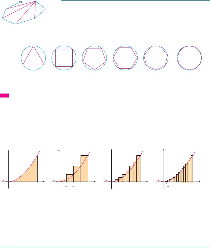
The origins of calculus go back at least 2500 years to the ancient Greeks, who found areas using the “method of exhaustion.” They knew how to ﬁnd the area A of any polygon by dividing it into triangles as in Figure 1 and adding the areas of these triangles.

It is a much more difﬁcult problem to ﬁnd the area of a curved ﬁgure. The Greek method of exhaustion was to inscribe polygons in the ﬁgure and circumscribe polygons about the ﬁgure and then let the number of sides of the polygons increase. Figure 2 illustrates this process for the special case of a circle with inscribed regular polygons.

A¢

A∞

Aß

A¶

A¡™

TEC In the Preview Visual, you can see how inscribed and circumscribed polygons approximate the area of a circle.

Let An be the area of the inscribed polygon with n sides. As n increases, it appears that An becomes closer and closer to the area of the circle. We say that the area of the circle is the limit of the areas of the inscribed polygons, and we write

A lim An

n l

The Greeks themselves did not use limits explicitly. However, by indirect reasoning, Eudoxus (ﬁfth century BC) used exhaustion to prove the familiar formula for the area of a circle: A r 2.

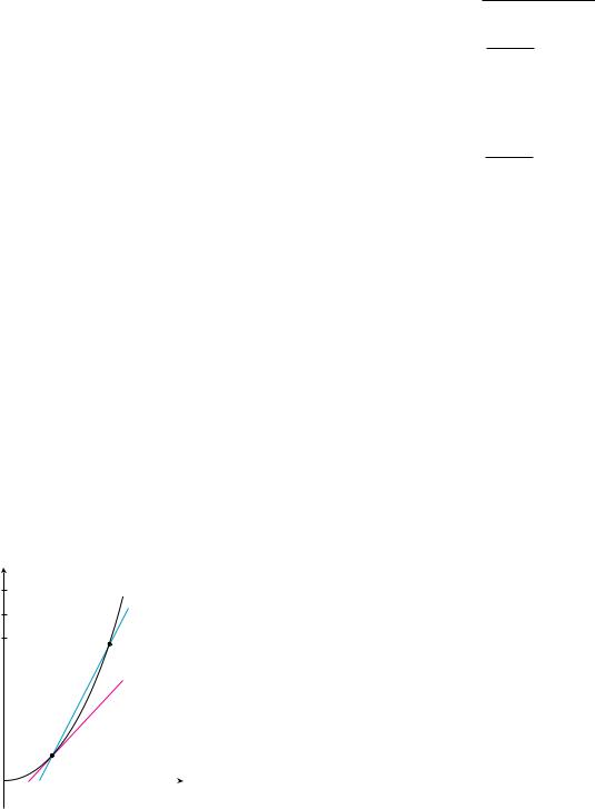
We will use a similar idea in Chapter 5 to ﬁnd areas of regions of the type shown in Figure 3. We will approximate the desired area A by areas of rectangles (as in Figure 4), let the width of the rectangles decrease, and then calculate A as the limit of these sums of areas of rectangles.

(1, 1)

y=≈

y
					(1, 1)
0	1	1	3	1	x
	4	2	4

FIGURE 3

FIGURE 4

y
		(1, 1)
0	1	x

y
			(1, 1)
0	1	1	x
	n

The area problem is the central problem in the branch of calculus called integral calculus. The techniques that we will develop in Chapter 5 for ﬁnding areas will also enable us to compute the volume of a solid, the length of a curve, the force of water against a dam, the mass and center of gravity of a rod, and the work done in pumping water out of a tank.

4 |||| A PREVIEW OF CALCULUS

y=ƒ

FIGURE 5

The tangent line at P

	Q{x, ƒ}
P{a,f(a)}	ƒ-f(a)
P{a,f(a)}
	x-a

0 a x x

FIGURE 6

The secant line PQ

FIGURE 7

Secant lines approaching the tangent line

THE TANGENT PROBLEM

Consider the problem of trying to ﬁnd an equation of the tangent line t to a curve with equation y f x at a given point P. (We will give a precise deﬁnition of a tangent line in Chapter 2. For now you can think of it as a line that touches the curve at P as in Figure 5.) Since we know that the point P lies on the tangent line, we can ﬁnd the equation of t if we know its slope m. The problem is that we need two points to compute the slope and we know only one point, P, on t. To get around the problem we ﬁrst ﬁnd an approximation to m by taking a nearby point Q on the curve and computing the slope mPQ of the secant line PQ. From Figure 6 we see that

1	mPQ	f x f a
		x a

Now imagine that Q moves along the curve toward P as in Figure 7. You can see that the secant line rotates and approaches the tangent line as its limiting position. This means that the slope mPQ of the secant line becomes closer and closer to the slope m of the tangent line. We write

m lim mPQ

Q lP

and we say that m is the limit of mPQ as Q approaches P along the curve. Since x approaches a as Q approaches P, we could also use Equation 1 to write

2	m lim	f x f a

	x la x a

Speciﬁc examples of this procedure will be given in Chapter 2.

The tangent problem has given rise to the branch of calculus called differential calculus, which was not invented until more than 2000 years after integral calculus. The main ideas behind differential calculus are due to the French mathematician Pierre Fermat (1601–1665) and were developed by the English mathematicians John Wallis (1616–1703), Isaac Barrow (1630–1677), and Isaac Newton (1642–1727) and the German mathematician Gottfried Leibniz (1646–1716).

The two branches of calculus and their chief problems, the area problem and the tangent problem, appear to be very different, but it turns out that there is a very close connection between them. The tangent problem and the area problem are inverse problems in a sense that will be described in Chapter 5.

VELOCITY

When we look at the speedometer of a car and read that the car is traveling at 48 mi h, what does that information indicate to us? We know that if the velocity remains constant, then after an hour we will have traveled 48 mi. But if the velocity of the car varies, what does it mean to say that the velocity at a given instant is 48 mi h?

In order to analyze this question, let’s examine the motion of a car that travels along a straight road and assume that we can measure the distance traveled by the car (in feet) at l-second intervals as in the following chart:

t Time elapsed (s)	0	1	2	3	4	5

d Distance (ft)	0	2	9	24	42	71

A PREVIEW OF CALCULUS |||| 5

As a ﬁrst step toward ﬁnding the velocity after 2 seconds have elapsed, we ﬁnd the average velocity during the time interval 2 t 4:

average velocity change in position time elapsed

42 9

4 2

16.5 ft s

Similarly, the average velocity in the time interval 2 t 3 is

average velocity 24 9 15 ft s 3 2

We have the feeling that the velocity at the instant t 2 can’t be much different from the average velocity during a short time interval starting at t 2. So let’s imagine that the distance traveled has been measured at 0.l-second time intervals as in the following chart:

t	2.0	2.1	2.2	2.3	2.4	2.5

d	9.00	10.02	11.16	12.45	13.96	15.80

Then we can compute, for instance, the average velocity over the time interval 2, 2.5 :

	average velocity			15.80 9.00			13.6 ft s
	average velocity						13.6 ft s
					2.5 2
The results of such calculations are shown in the following chart:

	Time interval	2, 3	2, 2.5			2, 2.4	2, 2.3	2, 2.2	2, 2.1

	Average velocity (ft s)	15.0	13.6			12.4	11.5	10.8	10.2

The average velocities over successively smaller intervals appear to be getting closer to a number near 10, and so we expect that the velocity at exactly t 2 is about 10 ft s. In

Chapter 2 we will deﬁne the instantaneous velocity of a moving object as the limiting value of the average velocities over smaller and smaller time intervals.

In Figure 8 we show a graphical representation of the motion of the car by plotting the distance traveled as a function of time. If we write d f t , then f t is the number of feet traveled after t seconds. The average velocity in the time interval 2, t is

					Q{t,f(t)}
							average velocity	change in position		f t f 2
								change in position		f t f 2

								time elapsed		t 2
								time elapsed		t 2
							which is the same as the slope of the secant line PQ in Figure 8. The velocity v when t 2

20							is the limiting value of this average velocity as t approaches 2; that is,
20
10			P{2,f(2)}				v lim		f t f 2
10

									t 2
0	1	2	3	4	5	t		t l2	t 2
0	1	2	3	4	5	t
							and we recognize from Equation 2 that this is the same as the slope of the tangent line to
FIGURE 8							the curve at P.

6 |||| A PREVIEW OF CALCULUS

Thus, when we solve the tangent problem in differential calculus, we are also solving problems concerning velocities. The same techniques also enable us to solve problems involving rates of change in all of the natural and social sciences.

THE LIMIT OF A SEQUENCE

In the ﬁfth century BC the Greek philosopher Zeno of Elea posed four problems, now known as Zeno’s paradoxes, that were intended to challenge some of the ideas concerning space and time that were held in his day. Zeno’s second paradox concerns a race between the Greek hero Achilles and a tortoise that has been given a head start. Zeno argued, as follows, that Achilles could never pass the tortoise: Suppose that Achilles starts at position a1 and the tortoise starts at position t1. (See Figure 9.) When Achilles reaches the point a2 t1, the tortoise is farther ahead at position t2. When Achilles reaches a3 t2 , the tortoise is at t3 . This process continues indeﬁnitely and so it appears that the tortoise will always be ahead! But this deﬁes common sense.

a¡	a™	a£	a¢	a∞ . . .
Achilles
tortoise	t¡	t™	t£	t¢ . . .
FIGURE 9	t¡	t™	t£	t¢ . . .

One way of explaining this paradox is with the idea of a sequence. The successive positions of Achilles a1, a2, a3, . . . or the successive positions of the tortoise t1, t2, t3, . . . form what is known as a sequence.

In general, a sequence an is a set of numbers written in a deﬁnite order. For instance, the sequence

{1, 12 , 13 , 14 , 15 , . . .}

can be described by giving the following formula for the nth term:

a¢ a£ a™

a¡

We can visualize this sequence by plotting its terms on a number line as in Fig-

01 ure 10(a) or by drawing its graph as in Figure 10(b). Observe from either picture that the

							(a)				terms of the sequence an 1 n are becoming closer and closer to 0 as n increases. In fact,
											we can ﬁnd terms as small as we please by making n large enough. We say that the limit
1											of the sequence is 0, and we indicate this by writing
1											of the sequence is 0, and we indicate this by writing
											lim	1	0
											lim		0
										n	n l	n
	1	2	3	4	5		6	7	8		n l	n


						(b)					In general, the notation
						(b)
FIGURE 10											lim an L
											n l

is used if the terms an approach the number L as n becomes large. This means that the numbers an can be made as close as we like to the number L by taking n sufﬁciently large.

A PREVIEW OF CALCULUS |||| 7

The concept of the limit of a sequence occurs whenever we use the decimal representation of a real number. For instance, if

then

a1 3.1

a2 3.14

a3 3.141

a4 3.1415

a5 3.14159

a6 3.141592

a7 3.1415926

lim an

n l

The terms in this sequence are rational approximations to .

Let’s return to Zeno’s paradox. The successive positions of Achilles and the tortoise form sequences an and tn , where an tn for all n. It can be shown that both sequences have the same limit:

lim an p lim tn

n l n l

It is precisely at this point p that Achilles overtakes the tortoise.

THE SUM OF A SERIES

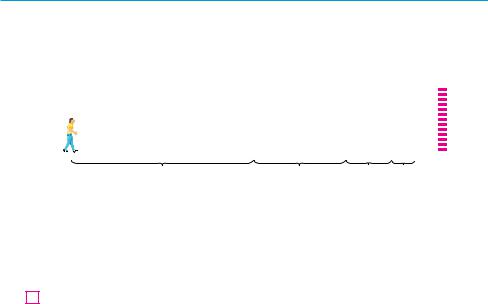
Another of Zeno’s paradoxes, as passed on to us by Aristotle, is the following: “A man standing in a room cannot walk to the wall. In order to do so, he would ﬁrst have to go half the distance, then half the remaining distance, and then again half of what still remains. This process can always be continued and can never be ended.” (See Figure 11.)













	1	1		1		1
FIGURE 11	2		4		8		16

Of course, we know that the man can actually reach the wall, so this suggests that perhaps the total distance can be expressed as the sum of inﬁnitely many smaller distances as follows:

3	1		1		1	1		1		1
3		2		4 8			16		2n
		2		4 8			16		2n

8 |||| A PREVIEW OF CALCULUS

Zeno was arguing that it doesn’t make sense to add inﬁnitely many numbers together. But there are other situations in which we implicitly use inﬁnite sums. For instance, in decimal notation, the symbol 0.3 0.3333 . . . means


		3		3		3		3
10								10,000
			100		1000
and so, in some sense, it must be true that
	3		3		3			3		1
10			100		1000		10,000
									3

More generally, if dn denotes the nth digit in the decimal representation of a number, then

0.d1d2 d3 d4 . . .	d1		d2		d3		dn
	10		102		103		10n

Therefore some inﬁnite sums, or inﬁnite series as they are called, have a meaning. But we must deﬁne carefully what the sum of an inﬁnite series is.

Returning to the series in Equation 3, we denote by sn the sum of the ﬁrst n terms of the series. Thus

s1 12 0.5

s2 12 14 0.75

s3 12 14 18 0.875

s4 12 14 18 161 0.9375

s5 12 14 18 161 321 0.96875

s6 12 14 18 161 321 641 0.984375

s7 12 14 18 161 321 641 1281 0.9921875

s10	21 41			1		0.99902344
s10	21 41			1024		0.99902344



s16		1	1			1	0.99998474

		2	4		216

Observe that as we add more and more terms, the partial sums become closer and closer to 1. In fact, it can be shown that by taking n large enough (that is, by adding sufﬁciently many terms of the series), we can make the partial sum sn as close as we please to the number 1. It therefore seems reasonable to say that the sum of the inﬁnite series is 1 and to write

1		1		1		1	1
2		4		8		2n

A PREVIEW OF CALCULUS |||| 9

In other words, the reason the sum of the series is 1 is that

lim sn 1

n l

In Chapter 11 we will discuss these ideas further. We will then use Newton’s idea of combining inﬁnite series with differential and integral calculus.

SUMMARY

We have seen that the concept of a limit arises in trying to ﬁnd the area of a region, the slope of a tangent to a curve, the velocity of a car, or the sum of an inﬁnite series. In each case the common theme is the calculation of a quantity as the limit of other, easily calculated quantities. It is this basic idea of a limit that sets calculus apart from other areas of mathematics. In fact, we could deﬁne calculus as the part of mathematics that deals with limits.

After Sir Isaac Newton invented his version of calculus, he used it to explain the motion of the planets around the sun. Today calculus is used in calculating the orbits of satellites and spacecraft, in predicting population sizes, in estimating how fast coffee prices rise, in forecasting weather, in measuring the cardiac output of the heart, in calculating life insurance premiums, and in a great variety of other areas. We will explore some of these uses of calculus in this book.

In order to convey a sense of the power of the subject, we end this preview with a list of some of the questions that you will be able to answer using calculus:

rays from sun		1.	How can we explain the fact, illustrated in Figure 12, that the angle of elevation
			from an observer up to the highest point in a rainbow is 42°? (See page 279.)
		2.	How can we explain the shapes of cans on supermarket shelves? (See page 333.)
	138°	3.	Where is the best place to sit in a movie theater? (See page 446.)
		3.
rays from sun	42°	4. How far away from an airport should a pilot start descent? (See page 206.)
rays from sun	42°	5.	How can we ﬁt curves together to design shapes to represent letters on a laser
		5.
			printer? (See page 639.)
observer		6.	Where should an inﬁelder position himself to catch a baseball thrown by an out-
FIGURE 12			ﬁelder and relay it to home plate? (See page 601.)
FIGURE 12

7.Does a ball thrown upward take longer to reach its maximum height or to fall back to its original height? (See page 590.)

1
FUNCTIONS	20
	20
AND MODELS	18
AND MODELS	16
	14
	12	20¡!N
		20¡!N
Hours	10	30¡!N
	8	40¡!N
	8	50¡!N
		50¡!N
	6	60¡!N
		60¡!N
	4
A graphical representation of a	2
function––here the number of	0
hours of daylight as a function	0	Mar. Apr. May June July Aug. Sept. Oct. Nov. Dec.
of the time of year at various
latitudes––is often the most
natural and convenient way to
represent the function.

The fundamental objects that we deal with in calculus are functions. This chapter prepares the way for calculus by discussing the basic ideas concerning functions, their graphs, and ways of transforming and combining them. We stress that a function can be represented in different ways: by an equation, in a table, by a graph, or in words. We look at the main types of functions that occur in calculus and describe the process of using these functions as mathematical models of real-world phenomena. We also discuss the use of graphing calculators and graphing software for computers.

<<< < Предыдущая 1 23 / 913 4 5 6 7 8 9 10 11 12 13 14 15 16 17 18 19 20 21 22 23 24 25 > Следующая >>>

Соседние файлы в предмете [НЕСОРТИРОВАННОЕ]

#
05.02.202055.36 Mб19Calculus, 7th Edition ( PDFDrive.com ).pdf
#
30.12.201945.82 Mб41Complete Solutions Manual for_ SINGLE VARIABLE CALCULUS Early Transcendentals 7th Edition by Stewart ( PDFDrive.com ).pdf
#
30.12.201918.09 Mб35[James_Stewart]_Single_Variable_Calculus_Early_Tr(BookFi).pdf