

- •CONTENTS
- •Preface
- •To the Student
- •Diagnostic Tests
- •1.1 Four Ways to Represent a Function
- •1.2 Mathematical Models: A Catalog of Essential Functions
- •1.3 New Functions from Old Functions
- •1.4 Graphing Calculators and Computers
- •1.6 Inverse Functions and Logarithms
- •Review
- •2.1 The Tangent and Velocity Problems
- •2.2 The Limit of a Function
- •2.3 Calculating Limits Using the Limit Laws
- •2.4 The Precise Definition of a Limit
- •2.5 Continuity
- •2.6 Limits at Infinity; Horizontal Asymptotes
- •2.7 Derivatives and Rates of Change
- •Review
- •3.2 The Product and Quotient Rules
- •3.3 Derivatives of Trigonometric Functions
- •3.4 The Chain Rule
- •3.5 Implicit Differentiation
- •3.6 Derivatives of Logarithmic Functions
- •3.7 Rates of Change in the Natural and Social Sciences
- •3.8 Exponential Growth and Decay
- •3.9 Related Rates
- •3.10 Linear Approximations and Differentials
- •3.11 Hyperbolic Functions
- •Review
- •4.1 Maximum and Minimum Values
- •4.2 The Mean Value Theorem
- •4.3 How Derivatives Affect the Shape of a Graph
- •4.5 Summary of Curve Sketching
- •4.7 Optimization Problems
- •Review
- •5 INTEGRALS
- •5.1 Areas and Distances
- •5.2 The Definite Integral
- •5.3 The Fundamental Theorem of Calculus
- •5.4 Indefinite Integrals and the Net Change Theorem
- •5.5 The Substitution Rule
- •6.1 Areas between Curves
- •6.2 Volumes
- •6.3 Volumes by Cylindrical Shells
- •6.4 Work
- •6.5 Average Value of a Function
- •Review
- •7.1 Integration by Parts
- •7.2 Trigonometric Integrals
- •7.3 Trigonometric Substitution
- •7.4 Integration of Rational Functions by Partial Fractions
- •7.5 Strategy for Integration
- •7.6 Integration Using Tables and Computer Algebra Systems
- •7.7 Approximate Integration
- •7.8 Improper Integrals
- •Review
- •8.1 Arc Length
- •8.2 Area of a Surface of Revolution
- •8.3 Applications to Physics and Engineering
- •8.4 Applications to Economics and Biology
- •8.5 Probability
- •Review
- •9.1 Modeling with Differential Equations
- •9.2 Direction Fields and Euler’s Method
- •9.3 Separable Equations
- •9.4 Models for Population Growth
- •9.5 Linear Equations
- •9.6 Predator-Prey Systems
- •Review
- •10.1 Curves Defined by Parametric Equations
- •10.2 Calculus with Parametric Curves
- •10.3 Polar Coordinates
- •10.4 Areas and Lengths in Polar Coordinates
- •10.5 Conic Sections
- •10.6 Conic Sections in Polar Coordinates
- •Review
- •11.1 Sequences
- •11.2 Series
- •11.3 The Integral Test and Estimates of Sums
- •11.4 The Comparison Tests
- •11.5 Alternating Series
- •11.6 Absolute Convergence and the Ratio and Root Tests
- •11.7 Strategy for Testing Series
- •11.8 Power Series
- •11.9 Representations of Functions as Power Series
- •11.10 Taylor and Maclaurin Series
- •11.11 Applications of Taylor Polynomials
- •Review
- •APPENDIXES
- •A Numbers, Inequalities, and Absolute Values
- •B Coordinate Geometry and Lines
- •E Sigma Notation
- •F Proofs of Theorems
- •G The Logarithm Defined as an Integral
- •INDEX
4.1
y
f(d)
f(a)
a 0 b |
c |
d |
e x |
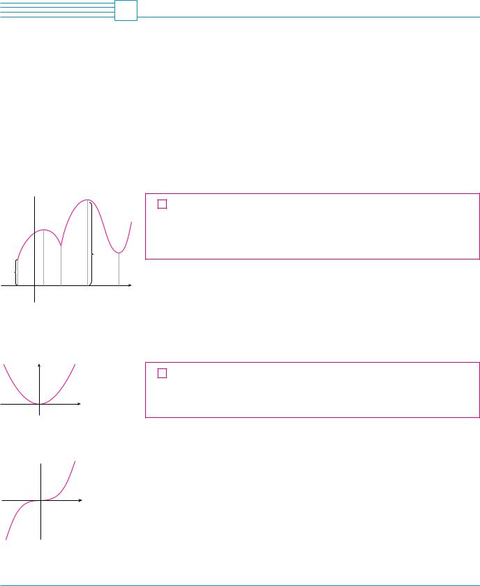
FIGURE 1
Minimum value f(a), maximum value f(d)
y
y=≈
0x
FIGURE 2
Minimum value 0, no maximum
y
y=þ
0x
FIGURE 3
No minimum, no maximum
MAXIMUM AND MINIMUM VALUES
Some of the most important applications of differential calculus are optimization problems, in which we are required to find the optimal (best) way of doing something. Here are examples of such problems that we will solve in this chapter:
■What is the shape of a can that minimizes manufacturing costs?
■What is the maximum acceleration of a space shuttle? (This is an important question to the astronauts who have to withstand the effects of acceleration.)
■What is the radius of a contracted windpipe that expels air most rapidly during a cough?
■At what angle should blood vessels branch so as to minimize the energy expended by the heart in pumping blood?
These problems can be reduced to finding the maximum or minimum values of a function. Let’s first explain exactly what we mean by maximum and minimum values.
1 DEFINITION A function f has an absolute maximum (or global maximum) at c if f !c" " f !x" for all x in D, where D is the domain of f. The number f !c" is called the maximum value of f on D. Similarly, f has an absolute minimum at c if f !c" % f !x" for all x in D and the number f !c" is called the minimum value of f on D. The maximum and minimum values of f are called the extreme values of f.
Figure 1 shows the graph of a function f with absolute maximum at d and absolute minimum at a. Note that !d, f !d"" is the highest point on the graph and !a, f !a"" is the lowest point. If we consider only values of x near b [for instance, if we restrict our attention to the interval !a, c"], then f !b" is the largest of those values of f !x" and is called a local maximum value of f. Likewise, f !c" is called a local minimum value of f because f !c" % f !x" for x near c [in the interval !b, d", for instance]. The function f also has a local minimum at e. In general, we have the following definition.
2 DEFINITION A function f has a local maximum (or relative maximum) at c if f !c" " f !x" when x is near c. [This means that f !c" " f !x" for all x in some open interval containing c.] Similarly, f has a local minimum at c if f !c" % f !x" when x is near c.
EXAMPLE 1 The function f !x" ! cos x takes on its (local and absolute) maximum value
of 1 infinitely many times, since cos 2n# ! 1 for any integer n and $1 % cos x % 1 for |
|
all x. Likewise, cos!2n ! 1"# ! $1 is its minimum value, where n is any integer. |
M |
EXAMPLE 2 If f !x" ! x2, then f !x" " f !0" because x2 " 0 for all x. Therefore f !0" ! 0
is the absolute (and local) minimum value of f. This corresponds to the fact that the |
|
origin is the lowest point on the parabola y ! x2. (See Figure 2.) However, there is no |
|
highest point on the parabola and so this function has no maximum value. |
M |
EXAMPLE 3 From the graph of the function f !x" ! x3, shown in Figure 3, we see that this function has neither an absolute maximum value nor an absolute minimum value. In fact, it has no local extreme values either. M
271
272 |||| CHAPTER 4 APPLICATIONS OF DIFFERENTIATION
|
|
y |
|
|
|
|
|
|
|
|
|
|
|
|
|
EXAMPLE 4 The graph of the function |
|
|
|
|
|
|
|
|
|
|
|
|
|
V |
|
||||
(_1,"37) |
|
|
y=3x$-16þ+18≈ |
|
|
f !x" ! 3x4 $ 16x3 ! 18x2 |
$1 % x % 4 |
||||||||||
|
|
|
|
|
|
|
|
|
|
|
|
|
|
|
is shown in Figure 4. You can see that f !1" ! 5 is a local maximum, whereas the |
||
|
|
|
|
|
|
|
|
|
|
|
|
|
|
|
absolute maximum is f !$1" ! 37. (This absolute maximum is not a local maximum |
||
|
|
|
(1,"5) |
|
|
|
|
|
|
|
because it occurs at an endpoint.) Also, f !0" ! 0 is a local minimum and f !3" ! $27 |
||||||
|
|
|
|
|
|
|
|
|
|
|
|
|
|
|
is both a local and an absolute minimum. Note that f |
has neither a local nor an absolute |
|
_ |
|
1 |
1 2 3 4 5 |
x maximum at x ! 4. |
M |
||||||||||||
|
|
|
|
|
|
|
|
|
|
|
|
|
|
|
|
We have seen that some functions have extreme values, whereas others do not. The |
|
|
|
|
(3,"_27) |
|
|
|
following theorem gives conditions under which a function is guaranteed to possess |
||||||||||
|
|
|
|
|
|
extreme values. |
|
||||||||||
|
|
|
|
|
|
|
|
|
|
|
|
|
|
|
|
|
|
FIGURE 4 |
|
|
|
|
|
|
|
|
|
|
|
|
|
3 THE EXTREME VALUE THEOREM If f is continuous on a closed interval #a, b$, |
|||
|
|
|
|
|
|
|
|
|
|
|
|
|
then f attains an absolute maximum value f !c" and an absolute minimum value |
||||
|
|
|
|
|
|
|
|
|
|
|
|
|
|
|
|
||
|
|
|
|
|
|
|
|
|
|
|
|
|
|
|
|
f !d" at some numbers c and d in #a, b$. |
|
|
|
|
|
|
|
|
|
|
|
|
|
|
|
|
|
|
|
The Extreme Value Theorem is illustrated in Figure 5. Note that an extreme value can be taken on more than once. Although the Extreme Value Theorem is intuitively very plausible, it is difficult to prove and so we omit the proof.
y |
y |
y |
FIGURE 5 |
0 a c |
d b x |
0 a c |
d=b x |
0 a cÁ d cª b x |
Figures 6 and 7 show that a function need not possess extreme values if either hypothesis (continuity or closed interval) is omitted from the Extreme Value Theorem.
y
3
1 
02 x
FIGURE 6
This function has minimum value f(2)=0, but no maximum value.
y
1 
02 x
FIGURE 7
This continuous function g has no maximum or minimum.
The function f whose graph is shown in Figure 6 is defined on the closed interval [0, 2] but has no maximum value. (Notice that the range of f is [0, 3). The function takes on values arbitrarily close to 3, but never actually attains the value 3.) This does not contradict the Extreme Value Theorem because f is not continuous. [Nonetheless, a discontinuous function could have maximum and minimum values. See Exercise 13(b).]
SECTION 4.1 MAXIMUM AND MINIMUM VALUES |||| 273
|
|
|
|
|
|
|
|
The function t shown in Figure 7 is continuous on the open interval (0, 2) but has nei- |
|
|
|
|
|
|
|
|
ther a maximum nor a minimum value. [The range of t is !1, )". The function takes on |
y |
|
|
|
|
|
|
|
arbitrarily large values.] This does not contradict the Extreme Value Theorem because the |
|
|
{c, f(c)} |
|
|
|
|
interval (0, 2) is not closed. |
|
|
|
|
|
|
||||
|
|
|
|
|
|
|
||
|
|
|
|
|
|
|
The Extreme Value Theorem says that a continuous function on a closed interval has a |
|
|
|
|
|
|
|
|
|
|
|
|
|
|
|
|
|
|
maximum value and a minimum value, but it does not tell us how to find these extreme |
|
|
|
|
|
|
|
|
values. We start by looking for local extreme values. |
|
|
|
|
|
|
|
|
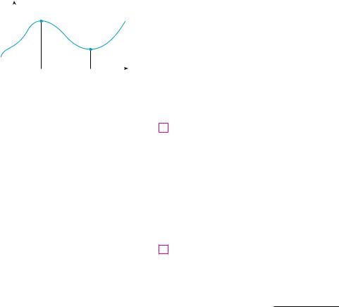
Figure 8 shows the graph of a function f with a local maximum at c and a local minimum |
|
|
|
|
|
{d, f(d)} |
|
||
|
|
|
|
|
|
|
x |
at d. It appears that at the maximum and minimum points the tangent lines are horizontal |
0 |
|
|
c |
|
d |
and therefore each has slope 0. We know that the derivative is the slope of the tangent line, |
||
|
|
|
|
|
|
|
|
so it appears that f &!c" ! 0 and f &!d" ! 0. The following theorem says that this is always |
|
|
|
|
|
|
|
|
|
FIGURE 8 |
|
|
|
|
true for differentiable functions. |
|||
N Fermat’s Theorem is named after Pierre Fermat (1601–1665), a French lawyer who took up mathematics as a hobby. Despite his amateur status, Fermat was one of the two inventors of analytic geometry (Descartes was the other). His methods for finding tangents to curves and maximum and minimum values (before the invention of limits and derivatives) made him a forerunner of Newton in the creation of differential calculus.
4 |
FERMAT’S THEOREM If f has a local maximum or minimum at c, and if f &!c" |
exists, then f &!c" ! 0. |
|
|
|
P R O O F |
Suppose, for the sake of definiteness, that f has a local maximum at c. Then, |
according to Definition 2, f !c" " f !x" if x is sufficiently close to c. This implies that if h is sufficiently close to 0, with h being positive or negative, then
f !c" " f !c ! h"
and therefore
5 |
f !c ! h" $ f !c" % 0 |
We can divide both sides of an inequality by a positive number. Thus, if h ( 0 and h is sufficiently small, we have
f !c ! h" $ f !c" % 0 h
Taking the right-hand limit of both sides of this inequality (using Theorem 2.3.2), we get
lim |
f !c ! h" $ f !c" |
% lim 0 ! 0 |
|||
|
|||||
h l0! |
h |
|
h l0! |
||
But since f &!c" exists, we have |
|
|
|
|
|
f &!c" ! lim |
f !c ! h" $ f !c" |
! lim |
f !c ! h" $ f !c" |
||
|
h |
||||
h l0 |
h |
|
h l0! |
||
and so we have shown that f &!c" % 0.
If h ' 0, then the direction of the inequality (5) is reversed when we divide by h:
|
|
f !c ! h" $ f !c" |
" 0 |
h ' 0 |
|
|
|
|
|
|
|||
|
|
h |
|
|
|
|
So, taking the left-hand limit, we have |
|
|
|
|
||
f &!c" ! lim |
f !c ! h" $ f !c" |
! lim |
f !c ! h" $ f !c" |
" 0 |
||
|
h |
|||||
|
h |
|||||
h l0 |
|
|
h l0$ |
|
||

274 |||| CHAPTER 4 APPLICATIONS OF DIFFERENTIATION
y
y=þ
0x
FIGURE 9 |
|
If Ä=þ, then f»(0)=0 but ƒ |
| |
has no maximum or minimum. |
y |
|
|
y=|x| |
0 |
x |
FIGURE 10
If Ä=|"x"|, then f(0)=0 is a minimum value, but f»(0) does not exist.
N Figure 11 shows a graph of the function f in Example 7. It supports our answer because
there is a horizontal tangent when x ! 1.5 and a vertical tangent when x ! 0.
3.5
We have shown that f &!c" " 0 and also that f &!c" % 0. Since both of these inequalities |
|
must be true, the only possibility is that f &!c" ! 0. |
|
We have proved Fermat’s Theorem for the case of a local maximum. The case of a |
|
local minimum can be proved in a similar manner, or we could use Exercise 76 to |
|
deduce it from the case we have just proved (see Exercise 77). |
M |
The following examples caution us against reading too much into Fermat’s Theorem. We can’t expect to locate extreme values simply by setting f &!x" ! 0 and solving for x.
EXAMPLE 5 If f !x" ! x3, then f &!x" ! 3x2, so f &!0" ! 0. But f has no maximum or minimum at 0, as you can see from its graph in Figure 9. (Or observe that x3 ( 0 for
x ( 0 but x3 ' 0 for x ' 0.) The fact that f &!0" ! 0 simply means that the curve y ! x3 has a horizontal tangent at !0, 0". Instead of having a maximum or minimum at !0, 0", the curve crosses its horizontal tangent there. M
EXAMPLE 6 The function f !x" ! & x & has its (local and absolute) minimum value at 0, but that value can’t be found by setting f &!x" ! 0 because, as was shown in Example 5 in Section 2.8, f &!0" does not exist. (See Figure 10.) M
WARNING Examples 5 and 6 show that we must be careful when using Fermat’s Theorem. Example 5 demonstrates that even when f &!c" ! 0 there need not be a maximum or minimum at c. (In other words, the converse of Fermat’s Theorem is false in general.) Furthermore, there may be an extreme value even when f &!c" does not exist (as in Example 6).
Fermat’s Theorem does suggest that we should at least start looking for extreme values
of f |
at the numbers c where f &!c" ! 0 or where f &!c" does not exist. Such numbers are |
|||
given a special name. |
|
|
||
|
|
|||
6 |
DEFINITION A critical number of a function f is a number c in the domain of |
|||
|
f |
such that either f &!c" ! 0 or f &!c" does not exist. |
|
|
|
|
|
|
|
|
EXAMPLE 7 Find the critical numbers of f !x" ! x3%5!4 $ x". |
|
|
|
V |
|
|
||
SOLUTION The Product Rule gives |
|
|
||
|
|
f &!x" ! x3%5!$1" ! !4 $ x"(53 x$2%5) ! $x3%5 ! |
3!4 $ x" |
|
|
|
5x2%5 |
||
|
|
|
||
|
|
|
|
|
! |
$5x ! 3!4 $ x" |
! |
12 $ 8x |
|
|
|
|
|
|
|
|
5x2%5 |
5x2%5 |
|
||
_0.5 |
|
|
|
5 |
[The same result could be obtained by first writing f !x" ! 4x3%5 |
$ x8%5.] Therefore |
||||
|
|
|
|
|
f &!x" ! 0 if 12 $ 8x ! 0, that is, x ! 23 , and f &!x" does not exist when x ! 0. Thus the |
|||||
_ |
|
2 |
|
critical numbers are 23 and 0. |
|
|
|
M |
||
|
|
In terms of critical numbers, Fermat’s Theorem can be rephrased as follows (compare |
||||||||
FIGURE 11 |
|
|||||||||
|
Definition 6 with Theorem 4): |
|
|
|
|
|||||
|
|
|
|
|
|
|
|
|
||
7 If f has a local maximum or minimum at c, then c is a critical number of f.
y
20 y=þ-3≈+1
(4,"17)
15
10
5
12
|
|
|
|
|
|
|
|
|
|
|
|
|
|
|
_ |
|
1 0 |
|
3 4 |
x |
|||||||||
_5 |
|
|
(2,"_3) |
|
|
|
|
|
|
|||||
|
|
|
|
|
|
|
|
|||||||
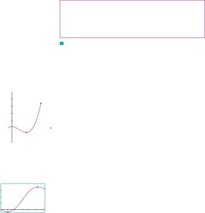
FIGURE 12
8
0 |
2π |
_1 |
|
FIGURE 13
SECTION 4.1 MAXIMUM AND MINIMUM VALUES |||| 275
To find an absolute maximum or minimum of a continuous function on a closed interval, we note that either it is local [in which case it occurs at a critical number by (7)] or it occurs at an endpoint of the interval. Thus the following three-step procedure always works.
THE CLOSED INTERVAL METHOD To find the absolute maximum and minimum values of a continuous function f on a closed interval #a, b$:
1.Find the values of f at the critical numbers of f in !a, b".
2.Find the values of f at the endpoints of the interval.
3.The largest of the values from Steps 1 and 2 is the absolute maximum value; the smallest of these values is the absolute minimum value.
V EXAMPLE 8 Find the absolute maximum and minimum values of the function
f !x" ! x3 $ 3x2 ! 1 $12 % x % 4
SOLUTION Since f is continuous on [$12 , 4], we can use the Closed Interval Method: f !x" ! x3 $ 3x2 ! 1
f &!x" ! 3x2 $ 6x ! 3x!x $ 2"
Since f &!x" exists for all x, the only critical numbers of f occur when f &!x" ! 0, that is, x ! 0 or x ! 2. Notice that each of these critical numbers lies in the interval ($12 , 4).
The values of |
f |
at these critical numbers are |
|
|
|
f !0" ! 1 |
f !2" ! $3 |
The values of |
f |
at the endpoints of the interval are |
|
|
|
f ($21 ) ! 81 |
f !4" ! 17 |
Comparing these four numbers, we see that the absolute maximum value is f !4" ! 17 and the absolute minimum value is f !2" ! $3.
Note that in this example the absolute maximum occurs at an endpoint, whereas the absolute minimum occurs at a critical number. The graph of f is sketched in Figure 12. M
If you have a graphing calculator or a computer with graphing software, it is possible to estimate maximum and minimum values very easily. But, as the next example shows, calculus is needed to find the exact values.
EXAMPLE 9
(a)Use a graphing device to estimate the absolute minimum and maximum values of the function f !x" ! x $ 2 sin x, 0 % x % 2#.
(b)Use calculus to find the exact minimum and maximum values.
SOLUTION
(a) Figure 13 shows a graph of f in the viewing rectangle #0, 2#$ by #$1, 8$. By moving the cursor close to the maximum point, we see that the y-coordinates don’t change very much in the vicinity of the maximum. The absolute maximum value is about 6.97 and it occurs when x ' 5.2. Similarly, by moving the cursor close to the minimum point, we see that the absolute minimum value is about $0.68 and it occurs when x ' 1.0. It is

276 |||| CHAPTER 4 APPLICATIONS OF DIFFERENTIATION
NASA
possible to get more accurate estimates by zooming in toward the maximum and minimum points, but instead let’s use calculus.
(b) The function f x x 2 sin x is continuous on 0, 2 . Since f x 1 2 cos x, we have f x 0 when cos x 12 and this occurs when x 3 or 5 3. The values of f at these critical points are
|
|
|
|
|
|
|
|
|
|
|
|
|
|
|||||
|
f 3 |
|
2 sin |
|
|
|
|
|
s3 0.684853 |
|
||||||||
|
3 |
|
3 |
3 |
|
|||||||||||||
|
|
5 |
|
|
|
5 |
|
|
5 |
|
|
|
||||||
|
|
|
|
|
|
|
|
|
||||||||||
and |
f 5 3 |
|
|
2 sin |
|
|
|
|
|
|
s3 6.968039 |
|
||||||
3 |
3 |
|
3 |
|
||||||||||||||
The values of f at the endpoints are |
|
|
|
|
|
|
|
|
|
|
|
|
|
|||||
|
f 0 0 |
and |
|
|
|
|
f 2 2 6.28 |
|
||||||||||
Comparing these four numbers and using the Closed Interval Method, we see that the |
|
|||||||||||||||||
absolute minimum value is f 3 3 s3 |
and the absolute maximum value is |
|
||||||||||||||||
f 5 3 5 3 s3 . The values from part (a) serve as a check on our work. |
M |
|||||||||||||||||
EXAMPLE 10 The Hubble Space Telescope was deployed on April 24, 1990, by the space shuttle Discovery. A model for the velocity of the shuttle during this mission, from liftoff at t 0 until the solid rocket boosters were jettisoned at t 126 s, is given by
v t 0.001302t 3 0.09029t 2 23.61t 3.083
(in feet per second). Using this model, estimate the absolute maximum and minimum values of the acceleration of the shuttle between liftoff and the jettisoning of the boosters.
SOLUTION We are asked for the extreme values not of the given velocity function, but rather of the acceleration function. So we first need to differentiate to find the acceleration:
a t v t d 0.001302t 3 0.09029t 2 23.61t 3.083 dt
0.003906t 2 0.18058t 23.61
We now apply the Closed Interval Method to the continuous function a on the interval 0 t 126. Its derivative is
a t 0.007812t 0.18058
The only critical number occurs when a t 0: |
|
|||
t1 |
|
0.18058 |
23.12 |
|
|
|
|||
|
0.007812 |
|
|
|
Evaluating a t at the critical number and at the endpoints, we have |
||||
a 0 23.61 |
a t1 21.52 |
a 126 62.87 |
||
So the maximum acceleration is about 62.87 ft s2 and the minimum acceleration is |
||||
about 21.52 ft s2. |
|
|
|
M |

SECTION 4.1 MAXIMUM AND MINIMUM VALUES |||| 277
4.1EXERCISES
1.Explain the difference between an absolute minimum and a local minimum.
2.Suppose f is a continuous function defined on a closed interval #a, b$.
(a)What theorem guarantees the existence of an absolute maximum value and an absolute minimum value for f ?
(b)What steps would you take to find those maximum and minimum values?
3– 4 For each of the numbers a, b, c, d, r, and s, state whether the function whose graph is shown has an absolute maximum or minimum, a local maximum or minimum, or neither a maximum
nor a minimum.
3. y |
4. y |
0 a b |
c d r |
s |
x |
0 a |
b |
c d r s x |
5–6 Use the graph to state the absolute and local maximum and minimum values of the function.
5. |
y |
|
|
|
1 |
|
y=Ä |
|
|
|
|
|
0 |
1 |
x |
6. |
y |
|
|
|
|
|
y=© |
|
1 |
|
|
|
0 |
1 |
x |
7–10 Sketch the graph of a function f that is continuous on [1, 5] and has the given properties.
7.Absolute minimum at 2, absolute maximum at 3, local minimum at 4
8.Absolute minimum at 1, absolute maximum at 5, local maximum at 2, local minimum at 4
9.Absolute maximum at 5, absolute minimum at 2, local maximum at 3, local minima at 2 and 4
10.f has no local maximum or minimum, but 2 and 4 are critical numbers
11.(a) Sketch the graph of a function that has a local maximum at 2 and is differentiable at 2.
(b)Sketch the graph of a function that has a local maximum at 2 and is continuous but not differentiable at 2.
(c)Sketch the graph of a function that has a local maximum at 2 and is not continuous at 2.
12.(a) Sketch the graph of a function on [$1, 2] that has an absolute maximum but no local maximum.
(b)Sketch the graph of a function on [$1, 2] that has a local maximum but no absolute maximum.
13.(a) Sketch the graph of a function on [$1, 2] that has an absolute maximum but no absolute minimum.
(b)Sketch the graph of a function on [$1, 2] that is discontinuous but has both an absolute maximum and an absolute minimum.
14.(a) Sketch the graph of a function that has two local maxima, one local minimum, and no absolute minimum.
(b)Sketch the graph of a function that has three local minima, two local maxima, and seven critical numbers.
15–28 Sketch the graph of f by hand and use your sketch to find the absolute and local maximum and minimum values of f. (Use the graphs and transformations of Sections 1.2 and 1.3.)
15. |
f !x" ! 8 |
$ 3x, |
x " 1 |
|
|
|
|
|
||||||
16. |
f !x" ! 3 |
$ 2x, |
x % 5 |
|
|
|
|
|
||||||
17. |
f !x" ! x |
2, |
|
0 ' x ' 2 |
|
|
|
|
|
|||||
18. |
f !x" ! x |
2, |
|
0 ' x % 2 |
|
|
|
|
|
|||||
19. |
f !x" ! x |
2, |
|
0 % x ' 2 |
|
|
|
|
|
|||||
20. |
f !x" ! x |
2, |
|
0 % x % 2 |
|
|
|
|
|
|||||
21. |
f !x" ! x |
2, |
|
$3 % x % 2 |
|
|
|
|
|
|||||
22. |
f !x" ! 1 ! !x ! 1"2, $2 % x ' 5 |
|
||||||||||||
23. |
f !x" ! ln x, |
0 ' x % 2 |
|
|
|
|
|
|||||||
24. |
f !t" ! cos t, |
|
$3#%2 % t % 3#%2 |
|
|
|
|
|||||||
25. |
f !x" ! 1 |
$ s |
|
|
|
|
|
|
|
|
|
|||
x |
|
|
|
|
|
|
|
|||||||
26. |
f !x" ! e x |
|
|
|
|
|
|
|
|
|
|
|
||
|
|
|
1 $ x |
if 0 % x ' 2 |
|
|
|
|
||||||
27. |
f !x" ! (2x $ 4 |
if 2 % x % 3 |
|
|
|
|
||||||||
|
|
|
4 |
$ x2 |
if $2 % x ' 0 |
|
|
|
|
|||||
28. |
f !x" ! (2x $ 1 |
if 0 % x % 2 |
|
|
|
|
||||||||
29– 44 Find the critical numbers of the function. |
|
|||||||||||||
29. |
f !x" ! 5x2 ! 4x |
|
|
30. |
f !x" ! x3 ! x2 |
$ x |
||||||||
31. |
f !x" ! x3 ! 3x2 |
$ 24x |
32. |
f !x" ! x3 ! x2 ! x |
||||||||||
33. |
s!t" ! 3t4 ! 4t3 |
$ 6t2 |
34. |
t!t" ! & 3t $ 4 & |
|
|||||||||
35. |
t!y" ! |
|
|
y $ 1 |
|
|
36. |
h! p" ! |
p $ 1 |
|
|
|||
y |
2 |
$ y ! 1 |
p2 ! 4 |
|
|
|||||||||

278 |||| CHAPTER 4 APPLICATIONS OF DIFFERENTIATION
37. |
h!t" ! t3%4 $ 2t1%4 |
38. |
t!x" ! s |
|
|
|
1 |
$ x2 |
|
||||
39. |
F!x" ! x4%5!x $ 4"2 |
40. |
t!x" ! x1%3 |
$ x$2%3 |
||
41. |
f !*" ! 2 cos * ! sin2* |
42. |
t!*" ! 4* $ tan |
* |
||
43. |
f!x" ! x2e$3x |
44. |
f! x" ! x$2 |
ln x |
|
|
|
|
|
|
|
|
|
;45– 46 A formula for the derivative of a function f is given. How many critical numbers does f have?
45. f &!x" ! 5e$0.1& x & sinx $ 1 |
46. |
f &!x" ! |
100 cos2 x |
$ 1 |
|
10 ! x2 |
|||||
|
|
|
|
||
|
|
|
|
|
47–62 Find the absolute maximum and absolute minimum values of f on the given interval.
47. |
f !x" ! 3x2 $ 12x ! 5, #0, 3$ |
|
||||||||||
48. |
f !x" ! x3 |
$ |
3x ! 1, |
#0, 3$ |
|
|||||||
49. |
f !x" ! 2x3 $ 3x2 |
$ 12x ! 1, #$2, 3$ |
||||||||||
50. |
f !x" ! x3 |
$ |
6x2 ! 9x ! 2, #$1, 4$ |
|||||||||
51. |
f !x" ! x4 |
$ |
2x2 ! 3, |
#$2, 3$ |
|
|||||||
52. |
f !x" ! !x2 $ 1"3, |
#$1, 2$ |
|
|||||||||
53. |
f !x" ! |
|
|
|
x |
|
|
, |
#0, 2$ |
|
||
x2 |
! |
1 |
|
|||||||||
54. |
f !x" ! |
x2 |
$ 4 |
, |
#$4, 4$ |
|
||||||
x2 ! 4 |
|
|||||||||||
55. |
f !t" ! ts |
|
|
|
, |
#$1, 2$ |
|
|||||
4 $ t2 |
|
|||||||||||
56. |
f !t" ! s |
|
|
!8 |
$ t", |
#0, 8$ |
|
|||||
t |
|
|||||||||||
|
3 |
|
|
|
|
|
|
|
|
|
|
|
57. |
f !t" ! 2cos t ! sin 2t, |
#0,#%2$ |
|
|||||||||
58. |
f !t" ! t ! cot!t%2", |
##%4, 7#%4 |
$ |
|||||||||
59. |
f !x" ! xe$x2%8, |
#$1, 4$ |
|
|||||||||
60. |
f !x" ! x $ ln x, |
|
[21 , 2] |
|
||||||||
61. |
f !x" ! ln!x2 ! x ! 1", #$1, 1$ |
|
||||||||||
62. |
f !x" ! e$x $ e$2x, |
#0, 1$ |
|
|||||||||
|
|
|
|
|
|
|
|
|
|
|
|
|
63.If a and b are positive numbers, find the maximum value of f !x" ! xa!1 $ x"b, 0 % x % 1.
;64. Use a graph to estimate the critical numbers of
&x3 $ 3x2 ! 2 & correct to one decimal place.f !x" !
;65–68
(a)Use a graph to estimate the absolute maximum and minimum values of the function to two decimal places.
(b)Use calculus to find the exact maximum and minimum values.
65.f !x" ! x5 $ x3 ! 2, $1 % x % 1
66. f !x" ! ex3$x, $1 % x % 0
67. f !x" ! xsx $ x2
68. f !x" ! x $ 2 cos x, $2 % x % 0
69.Between 0,C and 30,C, the volume V (in cubic centimeters) of 1 kg of water at a temperature T is given approximately by the formula
V ! 999.87 $ 0.06426T ! 0.0085043T 2 $ 0.0000679T 3
Find the temperature at which water has its maximum density.
70.An object with weight W is dragged along a horizontal plane by a force acting along a rope attached to the object. If the
rope makes an angle * with the plane, then the magnitude of the force is
+W
F ! + sin * ! cos *
where + is a positive constant called the coefficient of friction and where 0 % * % #%2. Show that F is minimized when tan * ! +.
71.A model for the US average price of a pound of white sugar from 1993 to 2003 is given by the function
S!t" ! $0.00003237t5 ! 0.0009037t4 $ 0.008956t3 ! 0.03629t2 $ 0.04458t ! 0.4074
where t is measured in years since August of 1993. Estimate the times when sugar was cheapest and most expensive during the period 1993–2003.
;72. On May 7, 1992, the space shuttle Endeavour was launched on mission STS-49, the purpose of which was to install a new perigee kick motor in an Intelsat communications satellite. The table gives the velocity data for the shuttle between liftoff and the jettisoning of the solid rocket boosters.
Event |
Time (s) |
Velocity (ft%s) |
|
|
|
Launch |
0 |
0 |
Begin roll maneuver |
10 |
185 |
End roll maneuver |
15 |
319 |
Throttle to 89% |
20 |
447 |
Throttle to 67% |
32 |
742 |
Throttle to 104% |
59 |
1325 |
Maximum dynamic pressure |
62 |
1445 |
Solid rocket booster separation |
125 |
4151 |
|
|
|
(a) Use a graphing calculator or computer to find the cubic polynomial that best models the velocity of the shuttle for the time interval t ! #0, 125$. Then graph this polynomial.
(b) Find a model for the acceleration of the shuttle and use it to estimate the maximum and minimum values of the acceleration during the first 125 seconds.
APPLIED PROJECT THE CALCULUS OF RAINBOWS |||| 279
73.When a foreign object lodged in the trachea (windpipe) forces a person to cough, the diaphragm thrusts upward causing an increase in pressure in the lungs. This is accompanied by a contraction of the trachea, making a narrower channel for the expelled air to flow through. For a given amount of air to escape in a fixed time, it must move faster through the narrower channel than the wider one. The greater the velocity of the airstream, the greater the force on the foreign object.
X rays show that the radius of the circular tracheal tube contracts to about two-thirds of its normal radius during a cough. According to a mathematical model of coughing, the velocity v of the airstream is related to the radius r of the trachea by the equation
v!r" ! k!r0 |
$ r"r2 21 r0 % r % r0 |
where k is a constant and r0 is the normal radius of the trachea. The restriction on r is due to the fact that the tracheal wall stiffens under pressure and a contraction greater than 12 r0 is prevented (otherwise the person would suffocate).
(a)Determine the value of r in the interval [12 r0, r0] at which v has an absolute maximum. How does this compare with experimental evidence?
(b)What is the absolute maximum value of v on the interval?
(c)Sketch the graph of v on the interval #0, r0 $.
74.Show that 5 is a critical number of the function
t!x" ! 2 ! !x $ 5"3
but t does not have a local extreme value at 5. 75. Prove that the function
f !x" ! x101 ! x51 ! x ! 1
has neither a local maximum nor a local minimum.
76.If f has a minimum value at c, show that the function t!x" ! $f !x" has a maximum value at c.
77.Prove Fermat’s Theorem for the case in which f has a local minimum at c.
78.A cubic function is a polynomial of degree 3; that is, it has the form f !x" ! ax3 ! bx2 ! cx ! d, where a " 0.
(a)Show that a cubic function can have two, one, or no critical number(s). Give examples and sketches to illustrate the three possibilities.
(b)How many local extreme values can a cubic function have?
|
A P P L I E D |
THE CALCULUS OF RAINBOWS |
|
P R O J E C T |
|
|
Rainbows are created when raindrops scatter sunlight. They have fascinated mankind since |
|
|
|
|
|
|
|
|
|
ancient times and have inspired attempts at scientific explanation since the time of Aristotle. In |
|
|
this project we use the ideas of Descartes and Newton to explain the shape, location, and colors |
|
|
of rainbows. |
Π|
A |
|
|
|
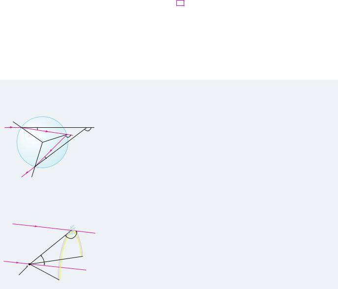
1. |
The figure shows a ray of sunlight entering a spherical raindrop at A. Some of the light is |
|
∫ |
|
B |
|
reflected, but the line AB shows the path of the part that enters the drop. Notice that the light |
|||
from |
|
|
D(Π) |
||||
|
∫ |
is refracted toward the normal line AO and in fact Snell’s Law says that sin - ! k sin /, |
|||||
sun |
|
O |
|
||||
|
|
∫ |
|
|
where - is the angle of incidence, / is the angle of refraction, and k ' 34 is the index of |
||
|
|
|
|
|
|
refraction for water. At B some of the light passes through the drop and is refracted into the |
|
|
|
∫ |
|
|
|
air, but the line BC shows the part that is reflected. (The angle of incidence equals the angle |
|
|
|
C |
|
|
|
of reflection.) When the ray reaches C, part of it is reflected, but for the time being we are |
|
to |
Π|
|
|
|
more interested in the part that leaves the raindrop at C. (Notice that it is refracted away |
||
observer |
|
|
|
|
from the normal line.) The angle of deviation D!-" is the amount of clockwise rotation that |
||
|
|
|
|
the ray has undergone during this three-stage process. Thus |
|||
Formation of the primary rainbow |
|||||||
|
|||||||
|
|
|
D!-" ! !- $ /" ! !# $ 2/" ! !- $ /" ! # ! 2- $ 4/ |
rays from sun |
|
|
Show that the minimum value of the deviation is D!-" ' 138, and occurs when - ' 59.4,. |
|
|
|
The significance of the minimum deviation is that when - ' 59.4, we have D&!-" ' 0, so |
|
|
|
.D%.- ' 0. This means that many rays with - ' 59.4, become deviated by approximately |
|
|
138¡ |
the same amount. It is the concentration of rays coming from near the direction of minimum |
|
|
deviation that creates the brightness of the primary rainbow. The figure at the left shows |
|
|
|
|
|
rays from sun |
42¡ |
|
that the angle of elevation from the observer up to the highest point on the rainbow is |
|
180, $ 138, ! 42,. (This angle is called the rainbow angle.) |
||
|
|
|
|
|
|
|
2. Problem 1 explains the location of the primary rainbow, but how do we explain the colors? |
observer |
|
|
Sunlight comprises a range of wavelengths, from the red range through orange, yellow, |