Добавил:

PavelEngineer Опубликованный материал нарушает ваши авторские права? Сообщите нам.

Вуз:

Севастопольский Государственный Университет

Предмет:

[НЕСОРТИРОВАННОЕ]

Файл:

[James_Stewart]_Single_Variable_Calculus_Early_Tr(BookFi).pdf

Скачиваний:

Добавлен:

30.12.2019

Размер:

18.09 Mб

Скачать

☆

<<< < Предыдущая 50 51 52 53 54 55 56 57 58 59 60 6162 / 9162 63 64 65 66 67 68 69 70 71 72 73 74 > Следующая >>>

572 |||| CHAPTER 9 DIFFERENTIAL EQUATIONS

(c)Make a rough sketch of a possible solution of this differential equation.

14.Suppose you have just poured a cup of freshly brewed coffee with temperature 95 C in a room where the temperature

is 20 C.

(a)When do you think the coffee cools most quickly? What happens to the rate of cooling as time goes by? Explain.

(b)Newton’s Law of Cooling states that the rate of cooling of

an object is proportional to the temperature difference between the object and its surroundings, provided that this difference is not too large. Write a differential equation that expresses Newton’s Law of Cooling for this particular situation. What is the initial condition? In view of your answer to part (a), do you think this differential equation is an appropriate model for cooling?

(c)Make a rough sketch of the graph of the solution of the initial-value problem in part (b).

9.2 DIRECTION FIELDS AND EULER’S METHOD

Unfortunately, it’s impossible to solve most differential equations in the sense of obtaining an explicit formula for the solution. In this section we show that, despite the absence of an explicit solution, we can still learn a lot about the solution through a graphical approach (direction ﬁelds) or a numerical approach (Euler’s method).

y
Slope at	Slope at	DIRECTION FIELDS
Slope at	Slope at
(⁄,›) is	(¤,ﬁ) is	Suppose we are asked to sketch the graph of the solution of the initial-value problem
⁄+›.	¤+ﬁ.		y 0 1
		y x y	y 0 1

0x We don’t know a formula for the solution, so how can we possibly sketch its graph? Let’s

think about what the differential equation means. The equation y x y tells us that the

FIGURE 1

slope at any point x, y on the graph (called the solution curve) is equal to the sum of the

x- and y-coordinates of the point (see Figure 1). In particular, because the curve passes

A solution of yª=x+y

through the point 0, 1 , its slope there must be 0 1 1. So a small portion of the solu-

tion curve near the point 0, 1 looks like a short line segment through 0, 1 with slope 1.

(See Figure 2.)

As a guide to sketching the rest of the curve, let’s draw short line segments at a num-

(0,1)

Slope at (0,1)

ber of points x, y with slope x y. The result is called a direction ﬁeld and is shown in

Figure 3. For instance, the line segment at the point 1, 2 has slope 1 2 3. The direc-

is 0+1=1.

tion ﬁeld allows us to visualize the general shape of the solution curves by indicating the

direction in which the curves proceed at each point.

FIGURE 2

Beginning of the solution curve

through (0,1)

(0,1)

FIGURE 3

FIGURE 4

Direction field for yª=x+y

The solution curve through (0,1)

SECTION 9.2 DIRECTION FIELDS AND EULER’S METHOD |||| 573

					Now we can sketch the solution curve through the point 0, 1 by following the direc-
				tion ﬁeld as in Figure 4. Notice that we have drawn the curve so that it is parallel to near-
				by line segments.
					In general, suppose we have a ﬁrst-order differential equation of the form
								y F x, y
				where F x, y is some expression in x and y. The differential equation says that the slope
				of a solution curve at a point x, y on the curve is F x, y . If we draw short line segments
				with slope F x, y at several points x, y , the result is called a direction ﬁeld (or slope
				ﬁeld). These line segments indicate the direction in which a solution curve is heading, so
				the direction ﬁeld helps us visualize the general shape of these curves.
		y		V EXAMPLE 1
		2		(a)	Sketch the direction ﬁeld for the differential equation y x 2 y 2 1.
				(b)	Use part (a) to sketch the solution curve that passes through the origin.
		1		SOLUTION
				SOLUTION
				(a)	We start by computing the slope at several points in the following chart:
_2	_1	0	1	2 x
		-1			x	2	1	0	1	2	2	1	0	1	2	. . .
		_2			y	0	0	0	0	0	1	1	1	1	1	. . .
		_2
FIGURE 5				y x 2 y 2 1		3	0	1	0	3	4	1	0	1	4	. . .
FIGURE 5

Now we draw short line segments with these slopes at these points. The result is the

y		direction ﬁeld shown in Figure 5.
2
2

(b)We start at the origin and move to the right in the direction of the line segment

1 (which has slope 1). We continue to draw the solution curve so that it moves parallel to the nearby line segments. The resulting solution curve is shown in Figure 6. Returning

			to the origin, we draw the solution curve to the left as well.			M
_2	_1 0	1	2 x
	-1			The more line segments we draw in a direction ﬁeld, the clearer the picture becomes.
	-1		Of course, it’s tedious to compute slopes and draw line segments for a huge number of

	_2		points by hand, but computers are well suited for this task. Figure 7 shows a more detailed,
	_2		computer-drawn direction ﬁeld for the differential equation in Example 1. It enables us to

FIGURE 6			draw, with reasonable accuracy, the solution curves shown in Figure 8 with y-intercepts
			2, 1, 0, 1, and 2.
				3		3
TEC Module 9.2A shows direction
ﬁelds and solution curves for a variety of
differential equations.
			_3	3	_3	3

FIGURE 7

FIGURE 8

574 \|\|\|\| CHAPTER 9	DIFFERENTIAL EQUATIONS
R		Now let’s see how direction ﬁelds give insight into physical situations. The simple elec-
		tric circuit shown in Figure 9 contains an electromotive force (usually a battery or gener-
E	L	ator) that produces a voltage of E t volts (V) and a current of I t amperes (A) at time t.
E	L	The circuit also contains a resistor with a resistance of R ohms ( ) and an inductor with
		an inductance of L henries (H).
		Ohm’s Law gives the drop in voltage due to the resistor as RI. The voltage drop due to
switch		the inductor is L dI dt . One of Kirchhoff’s laws says that the sum of the voltage drops is

FIGURE 9	equal to the supplied voltage E t . Thus we have
FIGURE 9
	1	L dI RI E t

which is a ﬁrst-order differential equation that models the current I at time t.

V EXAMPLE 2 Suppose that in the simple circuit of Figure 9 the resistance is 12 , the inductance is 4 H, and a battery gives a constant voltage of 60 V.

(a)Draw a direction ﬁeld for Equation 1 with these values.

(b)What can you say about the limiting value of the current?

(c)Identify any equilibrium solutions.

(d)If the switch is closed when t 0 so the current starts with I 0 0, use the direction ﬁeld to sketch the solution curve.

SOLUTION

(a) If we put L 4, R 12, and E t 60 in Equation 1, we get

4	dI	12I 60 or	dI	15 3I
	dt		dt

The direction ﬁeld for this differential equation is shown in Figure 10.

3 t

FIGURE 10

(b) It appears from the direction ﬁeld that all solutions approach the value 5 A, that is,

lim I t 5

t l

(c) It appears that the constant function I t 5 is an equilibrium solution. Indeed, we can verify this directly from the differential equation dI dt 15 3I. If I t 5, then the left side is dI dt 0 and the right side is 15 3 5 0.

SECTION 9.2 DIRECTION FIELDS AND EULER’S METHOD |||| 575

(d) We use the direction ﬁeld to sketch the solution curve that passes through 0, 0 , as shown in red in Figure 11.

I
6
4
2
0	1	2	3 t

FIGURE 11

Notice from Figure 10 that the line segments along any horizontal line are parallel. That is because the independent variable t does not occur on the right side of the equation I 15 3I. In general, a differential equation of the form

y f y

in which the independent variable is missing from the right side, is called autonomous.

For such an equation, the slopes corresponding to two different points with the same

y-coordinate must be equal. This means that if we know one solution to an autonomous

differential equation, then we can obtain inﬁnitely many others just by shifting the graph

of the known solution to the right or left. In Figure 11 we have shown the solutions

that result from shifting the solution curve of Example 2 one and two time units (namely,

solution curve

seconds) to the right. They correspond to closing the switch when t 1 or t 2.

y=L(x)

EULER’S METHOD

The basic idea behind direction ﬁelds can be used to ﬁnd numerical approximations to

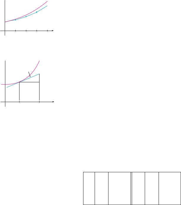
solutions of differential equations. We illustrate the method on the initial-value problem

that we used to introduce direction ﬁelds:

FIGURE 12

y x y

y 0 1

First Euler approximation

The differential equation tells us that y 0 0 1 1, so the solution curve has slope

1 at the point 0, 1 . As a ﬁrst approximation to the solution we could use the linear approx-

imation L x x 1. In other words, we could use the tangent line at 0, 1 as a rough

approximation to the solution curve (see Figure 12).

Euler’s idea was to improve on this approximation by proceeding only a short distance

along this tangent line and then making a midcourse correction by changing direction as

indicated by the direction ﬁeld. Figure 13 shows what happens if we start out along the

1.5

tangent line but stop when x 0.5. (This horizontal distance traveled is called the step

size.) Since L 0.5 1.5, we have y 0.5 1.5 and we take 0.5, 1.5 as the starting point

0.5

for a new line segment. The differential equation tells us that y 0.5 0.5 1.5 2, so

we use the linear function

FIGURE 13

Euler approximation with step size 0.5

y 1.5 2 x 0.5 2x 0.5

576 |||| CHAPTER 9 DIFFERENTIAL EQUATIONS

1
0	0.25	1 x

FIGURE 14

Euler approximation with step size 0.25

slope=F(x¸,y¸)

(⁄,›)

hF(x¸,y¸)

y¸

x¸

⁄

FIGURE 15

as an approximation to the solution for x 0.5 (the orange segment in Figure 13). If we decrease the step size from 0.5 to 0.25, we get the better Euler approximation shown in Figure 14.

In general, Euler’s method says to start at the point given by the initial value and proceed in the direction indicated by the direction ﬁeld. Stop after a short time, look at the slope at the new location, and proceed in that direction. Keep stopping and changing direction according to the direction ﬁeld. Euler’s method does not produce the exact solution to an initial-value problem—it gives approximations. But by decreasing the step size (and therefore increasing the number of midcourse corrections), we obtain successively better approximations to the exact solution. (Compare Figures 12, 13, and 14.)

For the general ﬁrst-order initial-value problem y F x, y , y x0 y0, our aim is to ﬁnd approximate values for the solution at equally spaced numbers x0, x1 x0 h, x2 x1 h, . . . , where h is the step size. The differential equation tells us that the slope at x0, y0 is y F x0, y0 , so Figure 15 shows that the approximate value of the solution when x x1 is

	y1 y0 hF x0, y0
Similarly,	y2	y1 hF x1, y1
In general,	yn	yn 1 hF xn 1, yn 1

EXAMPLE 3 Use Euler’s method with step size 0.1 to construct a table of approximate values for the solution of the initial-value problem

y x y

y 0 1

SOLUTION We are given that h 0.1, x0 0, y0 1, and F x, y x y. So we have

y1 y0 hF x0, y0 1 0.1 0 1 1.1

y2 y1 hF x1, y1 1.1 0.1 0.1 1.1 1.22

y3 y2 hF x2, y2 1.22 0.1 0.2 1.22 1.362

This means that if y x is the exact solution, then y 0.3 1.362.

Proceeding with similar calculations, we get the values in the table:

TEC	Module 9.2B shows how Euler’s	n	xn	yn	n	xn	yn
	Module 9.2B shows how Euler’s	n	xn	yn	n	xn	yn
method works numerically and visually
method works numerically and visually		1	0.1	1.100000	6	0.6	1.943122
for a variety of differential equations and		1	0.1	1.100000	6	0.6	1.943122
step sizes.		2	0.2	1.220000	7	0.7	2.197434
		3	0.3	1.362000	8	0.8	2.487178
		4	0.4	1.528200	9	0.9	2.815895
		5	0.5	1.721020	10	1.0	3.187485

For a more accurate table of values in Example 3 we could decrease the step size. But for a large number of small steps the amount of computation is considerable and so we need to program a calculator or computer to carry out these calculations. The following table shows the results of applying Euler’s method with decreasing step size to the initialvalue problem of Example 3.

SECTION 9.2 DIRECTION FIELDS AND EULER’S METHOD |||| 577

N Computer software packages that produce numerical approximations to solutions of differential equations use methods that are reﬁnements of Euler’s method. Although Euler’s method is simple and not as accurate, it is the basic idea on which the more accurate methods are based.

Step size	Euler estimate of y 0.5	Euler estimate of y 1

0.500	1.500000	2.500000
0.250	1.625000	2.882813
0.100	1.721020	3.187485
0.050	1.757789	3.306595
0.020	1.781212	3.383176
0.010	1.789264	3.409628
0.005	1.793337	3.423034
0.001	1.796619	3.433848

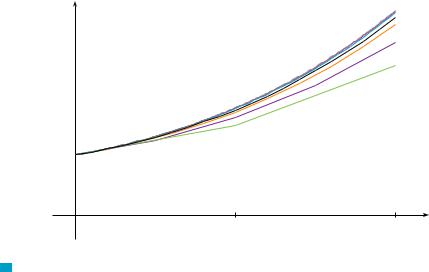
Notice that the Euler estimates in the table seem to be approaching limits, namely, the true values of y 0.5 and y 1 . Figure 16 shows graphs of the Euler approximations with step sizes 0.5, 0.25, 0.1, 0.05, 0.02, 0.01, and 0.005. They are approaching the exact solution curve as the step size h approaches 0.

FIGURE 16

Euler approximations approaching the exact solution

y
1
0	0.5	1	x
	0.5	1

V EXAMPLE 4 In Example 2 we discussed a simple electric circuit with resistance 12 , inductance 4 H, and a battery with voltage 60 V. If the switch is closed when t 0, we modeled the current I at time t by the initial-value problem

dI	15 3I	I 0 0
dt

Estimate the current in the circuit half a second after the switch is closed.

SOLUTION We use Euler’s method with F t, I 15 3I, t0 0, I0 0, and step size h 0.1 second:

I1 0 0.1 15 3 0 1.5

I2 1.5 0.1 15 3 1.5 2.55

I3 2.55 0.1 15 3 2.55 3.285

I4 3.285 0.1 15 3 3.285 3.7995

I5 3.7995 0.1 15 3 3.7995 4.15965

So the current after 0.5 seconds is

I 0.5 4.16 A

578 |||| CHAPTER 9 DIFFERENTIAL EQUATIONS

9.2E X E R C I S E S

A direction ﬁeld for the differential equation y y(1 41 y 2)

y x y 1

6. y sin x sin y

is shown.

(a) Sketch the graphs of the solutions that satisfy the given

initial conditions.

(i)

y 0 1

(ii)

y 0 1

(iii)

y 0 3

(iv)

y 0 3

(b) Find all the equilibrium solutions.

III

3 x

2.A direction ﬁeld for the differential equation y x sin y is shown.

(a)Sketch the graphs of the solutions that satisfy the given initial conditions.

(i)	y 0 1		(ii)	y 0 2			(iii) y 0
(iv)	y 0 4		(v)	y 0 5
(b) Find all the equilibrium solutions.
				y
				5
				4
				3
				2
				1
	_3	_2	_1	0	1	2	3 x

3–6 Match the differential equation with its direction ﬁeld (labeled I–IV). Give reasons for your answer.

3. y 2 y

4. y x 2 y

7.Use the direction ﬁeld labeled II (above) to sketch the graphs of the solutions that satisfy the given initial conditions.

(a) y 0 1

(b) y 0 2

8.Use the direction ﬁeld labeled IV (above) to sketch the graphs of the solutions that satisfy the given initial conditions.

(a) y 0 1

(b) y 0 0

9–10 Sketch a direction ﬁeld for the differential equation. Then use it to sketch three solution curves.

9. y 1 y	10. y x 2 y2

11–14 Sketch the direction ﬁeld of the differential equation. Then use it to sketch a solution curve that passes through the given point.

11.	y y 2x,	1, 0	12.	y 1 x y,	0, 0
13.	y y x y,	0, 1	14.	y x xy,	1, 0

CAS 15–16 Use a computer algebra system to draw a direction ﬁeld for the given differential equation. Get a printout and sketch on it the solution curve that passes through 0, 1 . Then use the CAS to draw the solution curve and compare it with your sketch.

15. y x 2 sin y 16. y x y2 4

CAS 17. Use a computer algebra system to draw a direction ﬁeld for the differential equation y y 3 4y. Get a printout and

SECTION 9.2 DIRECTION FILEDS AND EULER’S METHOD |||| 579

sketch on it solutions that satisfy the initial condition

y 0 c for various values of c. For what values of c does limt l y t exist? What are the possible values for this limit?

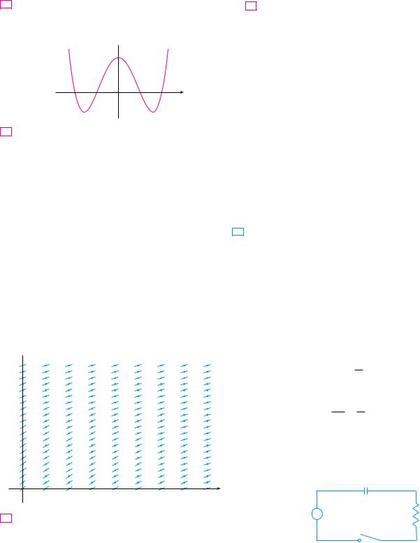
18.Make a rough sketch of a direction ﬁeld for the autonomous differential equation y f y , where the graph of f is as shown. How does the limiting behavior of solutions depend

on the value of y 0 ?

f(y)

_1 0

19.(a) Use Euler’s method with each of the following step sizes to estimate the value of y 0.4 , where y is the solution of the initial-value problem y y, y 0 1.

(i) h 0.4

(ii) h 0.2

(iii) h 0.1

(b)We know that the exact solution of the initial-value problem in part (a) is y e x. Draw, as accurately as you can, the graph of y e x, 0 x 0.4, together with the Euler approximations using the step sizes in part (a). (Your sketches should resemble Figures 12, 13, and 14.) Use your sketches to decide whether your estimates in part (a) are underestimates or overestimates.

(c)The error in Euler’s method is the difference between

the exact value and the approximate value. Find the errors

made in part (a) in using Euler’s method to estimate the true value of y 0.4 , namely e 0.4. What happens to the error each time the step size is halved?

20.A direction ﬁeld for a differential equation is shown. Draw, with a ruler, the graphs of the Euler approximations to the solution curve that passes through the origin. Use step sizes h 1 and h 0.5. Will the Euler estimates be underestimates or overestimates? Explain.

y 2

2 x

21.Use Euler’s method with step size 0.5 to compute the approx-

imate y-values y1, y2, y3, and y4 of the solution of the initialvalue problem y y 2x, y 1 0.

22. Use Euler’s method with step size 0.2 to estimate y 1 , where y x is the solution of the initial-value problem y 1 x y, y 0 0.

23.Use Euler’s method with step size 0.1 to estimate y 0.5 , where y x is the solution of the initial-value problem y y x y, y 0 1.

24.(a) Use Euler’s method with step size 0.2 to estimate y 1.4 , where y x is the solution of the initial-value problem y x xy, y 1 0.

(b)Repeat part (a) with step size 0.1.

;25. (a) Program a calculator or computer to use Euler’s method to compute y 1 , where y x is the solution of the initialvalue problem


	dy	3x 2 y 6x 2			y 0 3
		3x 2 y 6x 2			y 0 3
	dx
(i) h 1			(ii)	h 0.1
(iii) h 0.01			(iv)	h 0.001

(b)Verify that y 2 e x3 is the exact solution of the differential equation.

(c)Find the errors in using Euler’s method to compute y 1 with the step sizes in part (a). What happens to the error when the step size is divided by 10?

CAS 26. (a) Program your computer algebra system, using Euler’s method with step size 0.01, to calculate y 2 , where y is the solution of the initial-value problem

y x 3 y 3

y 0 1

(b)Check your work by using the CAS to draw the solution curve.

27.The ﬁgure shows a circuit containing an electromotive force, a capacitor with a capacitance of C farads (F), and a resistor

with a resistance of R ohms ( ). The voltage drop across the capacitor is Q C, where Q is the charge (in coulombs), so in this case Kirchhoff’s Law gives

RI Q E t

But I dQ dt, so we have

RdQ 1 Q E t dt C

Suppose the resistance is 5 , the capacitance is 0.05 F, and a battery gives a constant voltage of 60 V.

(a)Draw a direction ﬁeld for this differential equation.

(b)What is the limiting value of the charge?

<<< < Предыдущая 50 51 52 53 54 55 56 57 58 59 60 6162 / 9162 63 64 65 66 67 68 69 70 71 72 73 74 > Следующая >>>

Соседние файлы в предмете [НЕСОРТИРОВАННОЕ]

#
05.02.202055.36 Mб19Calculus, 7th Edition ( PDFDrive.com ).pdf
#
30.12.201945.82 Mб41Complete Solutions Manual for_ SINGLE VARIABLE CALCULUS Early Transcendentals 7th Edition by Stewart ( PDFDrive.com ).pdf
#
30.12.201918.09 Mб35[James_Stewart]_Single_Variable_Calculus_Early_Tr(BookFi).pdf